---
tags: NCTU_course, DLSR, NVIDIA
---

<center>DLSR Final Project Report</center>
=
<center>Group 1 | 0856044 孫嘉妤 0756162 謝季霖</center>

## Introduction
The topic of our final project is to perform **object detection** on **NEU surface defect database**[[1]](http://faculty.neu.edu.cn/yunhyan/NEU_surface_defect_database.html). NEU surface defect database is a dataset that contains six kinds of typical surface defects, and each defect includes 300 samples.


We choose **YOLOv3** [[2]](https://arxiv.org/abs/1804.02767) as our model, and implement our project based on the repository **PyTorch-YOLOv3** [[3]](https://github.com/eriklindernoren/PyTorch-YOLOv3).

In this project, we have two primary goals:

1. Increase the **mAP (Mean Average Precision)** of the object detection model. The AP is computed by the area under the precision-recall curve, and in our project, the true positive is defined by **IoU > 0.5** (IoU = the intersection over union of the prediction and the ground truth bounding boxes). We use several training techniques to improve the AP and the detailed information is described in the section "Improve Training".
2. Accelerate the speed of inference. We improve inference efficiency by **deploying on TensorRT**.

### Data Preprocessing

#### Create Datasets
Since **NEU surface defect database** only includes images & annotations, we separate the original data into three datasets (training/validation/ testing). We randomly seperate the data and ensure that the number of each class is the same. The ratio of the number of data of three datasets is `6:2:2`.

#### Convert Annotations to YOLO Format
NEU surface defect database provides **PASCAL VOC** [[4]](https://pjreddie.com/media/files/VOC2012_doc.pdf) format annotations. To apply YOLO on our data, first, we need to convert the annotations into **YOLO format**.

PASCAL VOC format represents the bounding box by the top-left coordinate and the bottom-right coordinate $(x_{top-left},\ y_{top-left}),\ (x_{bottom-right},\ y_{bottom-right})$ and stores the data in XML format. On the other hand, YOLO format represents the bounding box by the center and the height and weight $(x_{center},\ y_{center},\ weight,\ height)$.

> source code: `data_process/prepare_data.ipynb`.

## Training Improvement

### Data Augmentation - Heavy Augmentation

In the beginning, we simply applied several common data augmentation on our training data. The augmentations are `Gaussian blur`, `flip (vertical & horizontal)`, `rotation`, `dropout`, `noise`, and `hue/saturation` adjustment. We use **imgaug**[[5]](https://github.com/aleju/imgaug) as our implementation. The detailed setting and the implementation source code lists as follow:

self.aug = iaa.Sequential([
    iaa.Sometimes(0.25, iaa.GaussianBlur(sigma=(0, 3.0))),
    iaa.Sometimes(0.25, iaa.Fliplr(0.25)),
    iaa.Sometimes(0.25, iaa.Flipud(0.25)), 
    iaa.Sometimes(0.25, iaa.Affine(rotate=(-15, 15), mode='symmetric')), 
    iaa.Sometimes(0.25,
        iaa.OneOf([iaa.Dropout(p=(0, 0.25)),
        iaa.CoarseDropout((0.0, 0.05), size_percent=(0.02, 0.25))])),
    iaa.Sometimes(0.25, iaa.SaltAndPepper(0.5)),
    iaa.Sometimes(0.25, 
        iaa.AddToHueAndSaturation(value=(-20, 20), per_channel=True))
    ])

However, we did not get a worse result `AP = baseline-11%` after applying the heavy augmentation. We then visualized our augmentation results:


From the above pictures, we can observe that the blur & noise damage the structure of the original data, and the defect (crazing) became unrecognizable. Therefore, we adjust the augmentation settings several times and eventually achieved a better AP.

### Data Augmentation - Lite Augmentation
After several adjustments, our augmentation changes to the following settings:

self.aug = iaa.Sequential([
    iaa.Sometimes(0.25, iaa.Fliplr(0.5)),
    iaa.Sometimes(0.25, iaa.Flipud(0.5)), 
    iaa.Sometimes(0.1, iaa.Affine(rotate=(-15, 15), mode='symmetric')), 
    iaa.Sometimes(0.1,
        iaa.OneOf([iaa.Dropout(p=(0, 0.1)),
        iaa.CoarseDropout((0.0, 0.05), size_percent=(0.01, 0.1))])),
    iaa.Sometimes(0.1, iaa.SaltAndPepper(0.1))
])

The main difference between the lite augmentation and the heavy augmentation are:
1. The probability of applying augmentation is reduced from `0.25` to `0.1` (except flip), and the degree of each augmentation is lowered (such as the angle of rotation).
2. Augmentations related to `blur`, `massive noise (SaltAndPepper)` and `Hue/Saturation` are removed. We excluded the former due to the excessive noise, and excluded the former since our datasets are monochrome.


The above picture is the visualized result of the enhanced augmentation, and the mAP of lite augmentation is `baseline+2.3%`.

> source code: `utils/datasets.py`

### Misclassified Data Analysis & Image Processing
After applying augmentation, we do some statistical analysis and notice that the detection ratio & AP of `crazing` and `pitted_surface` are lower than other classes.


To improve the AP of these two classes, we observe the misclassified images (red bounding box = ground truth) and try to apply the image processing that can `highlight the edges and fine details` of the image.


#### Sharpen
We apply the `sharpen` as a preprocessing, that is, the sharpening effects will be applied to all the training and testing. The `sharpen` effect is also implemented by imgaug[[5]](https://github.com/aleju/imgaug). Sharpen implementation:

class SharpenTransform:
  def __init__(self):
    self.aug = iaa.Sequential([
        iaa.Sharpen(alpha=(0.75, 0.75), lightness=(1.25, 1.25))
    ])
      
  def __call__(self, img):
    img = np.array(img)
    out = self.aug.augment_image(img)
    out = PIL.Image.fromarray(out.astype('uint8'), 'RGB')
    return out

However, we do not get a better result by sharpening processing. The mAP of evaluation set becomes `baseline-1.8%` (but the mAP of validation set = `baseline+3.1%`). Our conjecture is: the working mechanism of ML-based models (especially CNN models) may be different from our intuition or human visual system. Although the edge looks more apparent, some subtle information may be ruined due to the sharpening operation. Besides, other techniques such as concatenating the processed data after the original data may get better results. We have not implemented such methods since it is more complicated to design for object detection models.

> source code: `utils/datasets.py`

### Adjust Anchor Boxes
YOLO performs predictions from a pre-determined set of boxes with particular height-width[[6]](https://github.com/pjreddie/darknet/issues/568), which is the so-called `anchor boxes`. Nevertheless, the default set of the anchor boxes may not fit the custom training data. Hence, we redefine the size of anchor boxes according to the object sizes of our dataset. We use `K-means clustering` to compute the new anchor boxes (the center of each cluster will become the new anchor box size).


The above is our clustering results. We cluster the bounding sizes by weight & height and get 9 sizes of bounding boxes (the default number of YOLO).

After adjusting anchor box sizes, the evaluation mAP increases to `baseline+3.1%` (validation mAP = `baseline+5.5%`).

> source code: `data_process/anchor_box.ipynb`

### Loss Function Enhancement
IoU (Intersection over Union) is a common metric of object detection tasks.


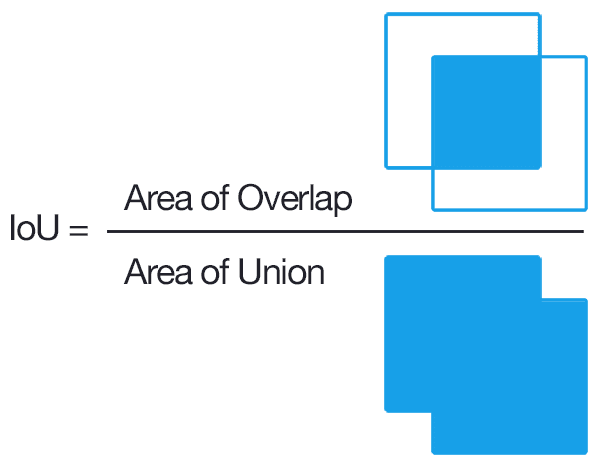
The figure[[7]](https://www.pyimagesearch.com/2016/11/07/intersection-over-union-iou-for-object-detection/) shows the definition of IoU: `the overlap between the prediction and the ground-truth` divides `the union of the prediction and the ground-truth`.

IoU is a straightforward and efficient metric: it is simple to compute and has the property of scale invariance (focuses on the area of the shapes, no matter their size)[[8]](https://giou.stanford.edu/). Nevertheless, recent research [[8]](https://giou.stanford.edu/GIoU.pdf)[[9]](https://arxiv.org/abs/1911.08287) indicates that there are several issues of using IoU as a metric. For instance:

* If the prediction and the ground truth bounding boxes do not overlap, the value of IoU = 0, which means that the following cases give the same loss value and can't benefit the training.


* Not sensitive to different aligned orientations (the IoU of the following cases are the same).


To solve the mentioned problems, we enhance the loss function by replacing IoU with GIoU (Generalized Intersection over Union)[[8]](https://giou.stanford.edu/). The concept of GIoU is `adding a penalty term` to suppress the area which should not be bounded. The image of the left[[10]](https://medium.com/@jacksonchou/distance-iou-loss-faster-and-better-learning-for-box-regression-9df8fc627e8) illustrates the main component of GIoU:


The loss function using GIoU can be denoted as: $\mathcal{L}_{GIoU}=1-IoU+\frac{\mid C-B\cup B^{gt} \mid}{\mid C \mid}$

Where $C$ is the smallest convex hull that encloses both $B$ (prediction bounding box) and $B^{gt}$ (ground-truth bounding box), and $\frac{\mid C-B\cup B^{gt} \mid}{\mid C \mid}$ is the mentioned `penalty term`. The above gives an example: if $C$ is larger than the value of $\mathcal{L}_{GIoU}$ becomes higher. Hence the right case will cause a higher loss than the left case.

#### Implementation
To apply GIoU to our project (the **PyTorch-YOLOv3** repository[[3]](https://github.com/eriklindernoren/PyTorch-YOLOv3)), we replace the original IoU function (`bbox_iou()` in `utils/utils.py`) with our GIoU version `bbox_giou()`. We refer to [[11]](https://zhuanlan.zhihu.com/p/94799295) and implement the GIoU function. The following is the code segment (some detailed operations are removed) of our GIoU implementation.
> complete source code: `utils/utils.py`

# compute C
area_C = (max(x1_pred,x2_pred,x1_gt,x2_gt)
        -min(x1_pred,x2_pred,x1_gt,x2_gt))*(max(y1_pred,y2_pred,y1_gt,y2_gt)
        -min(y1_pred,y2_pred,y1_gt,y2_gt))

# compute Union & Overlap
area_pred = (x2_pred-x1_pred)*(y1_pred-y2_pred)
area_gt = (x1_gt-x2_gt)*(y1_gt-y2_gt)
sum_area = area_pred + area_gt

w1 = x2_pred - x1_pred
w2 = x2_pred - x1_pred
h1 = y1_pred - y2_pred
h2 = y1_gt - y2_gt

W = min(x1_pred,x2_pred,x1_gt,x2_gt) + w1 + w2 - max(x1_pred,x2_pred,x1_gt,x1_gt)
H = min(y1_pred,y2_pred,y1_gt,y2_gt) + h1 + h2 - max(y1_pred,y2_pred,y1_gt,y2_gt)

Area = W*H
add_area = sum_area - Area

# get GIoU
end_area = (area_C - add_area)/area_C
giou = iou - end_area

### Experiments & Ablation Study

Here we summarize the results of experiments on the evaluation set:

| | Augment | Anchor Box | GIoU | Result (mAP) |
| -------- | -------- | -------- | -------- | -------- |
| Baseline | | | | 0.665 |
| Aug |v | | | 0.688 (+2.3%) |
| Anchor Box | | v | | 0.680 (+1.5%) |
| GIoU | | | v | 0.704 (+3.9%) |
| Aug + Anchor | v | v | | 0.693 (+2.8%) |
| Aug + GIoU | v | | v | 0.701 (+3.6%) |
| Anchor + GIoU | | v | v | 0.679 (+1.4%) |
| All | v | v | v | 0.711 (+4.6%) |

(abbreviations: aug/augment=data augmentation; anchor box=adjust anchor box sizes; GIoU=use GIoU instead of IoU)

From the experiment results, our observations and brief conclusions are: each technique can improve the mAP of our model. Furthermore, the experiment that applies all the techniques leads to the best mAP.

## TensorRT Deployment

### Environment
* CPU: Intel(R) Core(TM) i7-8700 CPU @ 3.20GHz (6C 12T)
* GPU: RTX 2060 SUPER
* Docker image: (Nvidia NGC) `nvcr.io/nvidia/pytorch:20.01-py3`
* CUDA version: 10.2
* TensorRT version: 7.0.0
* PyTorch version: 1.4.0

### Model conversion
#### Save Darknet weight from eriklindernoren/PyTorch-YOLOv3
According to the implementation of **PyTorch-YOLOv3**[[3]](https://github.com/eriklindernoren/PyTorch-YOLOv3), we can save weights of our PyTorch model in Darknet format using `save_darknet_weights` function from `class Darknet`, which is the first step of our TensorRT deployment for the YOLOv3 model.

#### Darknet to ONNX
After saving our PyTorch YOLOv3 model in Darknet format, the next step is to construct the ONNX graph with the Darknet config and weights, since ONNX is one of the acceptable model formats in TensorRT. Here we modified the sample code `yolov3_to_onnx.py` from NVIDIA, changed the model I/O, set correct output dimension, and fixed some bugs in the code.

#### ONNX to TensorRT
To successfully deploy the YOLOv3 model to TensorRT, it's necessary to check each layer in YOLOv3 model architecture and find which layer is unsupported in TensorRT. After the examination, we can observe that lots of operations used in YOLOv3 are Convolution, BatchNormalization, or LeakyRelu, which can be parsed and deployed to TensorRT directly. However, the detection layer (YOLO layer) in the model is not. To solve this issue, a simple solution is to only convert the YOLOv3 backbone to ONNX and TensorRT and implement the YOLO layer as part of postprocessing.

### Preprocessing
We implement the same preprocessing flow as PyTorch version, which consists of the following operations:
* Load images with Pillow `Image.open()`
* Resize to 416\*416 with nearest interpolate method
* Perform normalization and convert to 1D Numpy array
* Move to GPU memory for inference

### Postprocessing

#### Implementation of YOLO layer
After inferencing with TensorRT execution context, we will get three output arrays with different scales. The first thing we have to do in postprocessing is to reproduce the detection layer of YOLOv3, and apply it to these three output arrays to get real bounding-box coordinate information. The formula below shows what a detection layer does, for instance, we have to apply sigmoid, calculate exponential, multiply by anchor dimensions, and add corresponding grid coordinates.


#### Bounding boxes filtering
Since a one-stage object detection model predicts bounding boxes on each grid of feature maps, there are a huge number of objects will be predicted. However, only partial output objects have high object confidence, the others usually have less than 1% instead. For the purpose of getting a suitable result, it's required to filter these output proposals. Thus, we assign an object confidence threshold, and only choose objects which have higher object confidence than this threshold as our result.

#### Non-Maximum Suppression (NMS)
This step is used to filter repeated bounding boxes. As the figure below, sometimes both of the two bounding boxes have high object confidence, but they are overlapped --- that is, only one object exists actually. To deal with this condition, the Non-Maximum Suppression algorithm will filter objects according to their IoU and scores, and discard objects which have high IoU with the other but relative lower confidence.

### Visualization
The figures are the prediction result of `patches_93` in PyTorch and our TensorRT implementation. We have validated that the average difference of output arrays between PyTorch and TensorRT is less than 0.001.


### Benchmark

#### Perform inference on our NEU test dataset (360 images)
The table shows the performance of our model running on PyTorch and TensorRT respectively.
First, we built the TensorRT engine with original precision (FP32), and calculate the latency and the FPS. However, we only got about 5% performance improvement. Furthermore, we also tried to build a TensorRT engine with FP16 precision, and we got 45% performance improvement this time. The main reason for this outcome is due to the different optimization for FP32 and FP16 of Nvidia. When we use FP16, that means we only need half of digits compared with FP32. In addition, since Nvidia support this kind of operation, we can benefit from using FP16 and get a better performance improvement in the end.

| | Average Latency | FPS |
| ------ | ------ | ------ |
| PyTorch | 18.55 ms | 53.91 |
| TensorRT FP32 | 17.01 ms | 58.78 |
| TensorRT FP16 | 10.09 ms | 99.14 |

#### Discussion of postprocessing performance in PyTorch and TensorRT
Our postprocessing includes YOLO layer and NMS. In the table below, we can see that the postprocessing in PyTorch is faster. The main reason is that the YOLO layer and NMS in PyTorch’s implementation are constructed with lots of torch operations, which are running on CUDA devices. However, in our TensorRT implementation, the YOLO layer and NMS are not part of our TensorRT engine, thus they are running on the host. If we want to solve this issue, a TensoRT custom plugin for YOLO layer may be a good solution.

| | Average Latency |
| ------ | ------ |
| PyTorch | 2.39 ms |
| TensorRT FP32 | 3.64 ms |
| TensorRT FP16 | 3.66 ms |

## Reference
1. Song, Ke-Chen & Shaopeng, Hu & Yan, Y.. (2014). Automatic recognition of surface defects on hot-rolled steel strip using scattering convolution network. Journal of Computational Information Systems. 10. 3049-3055. 10.12733/jcis10026.
2. Redmon, Joseph & Farhadi, Ali. (2018). YOLOv3: An Incremental Improvement.
3. Erik Linder-Norén, PyTorch-YOLOv3, (2018), GitHub repository, https://github.com/eriklindernoren/PyTorch-YOLOv3
4. Everingham, Mark & Van Gool, Luc & Williams, Christopher & Winn, John & Zisserman, Andrew. (2010). The Pascal Visual Object Classes (VOC) challenge. International Journal of Computer Vision. 88. 303-338. 10.1007/s11263-009-0275-4.
5. Alexander B. Jung et al., imgaug, (2018), GitHub repository, https://github.com/aleju/imgaug
6. vkmenon, “Can someone clarify the anchor box concept used in Yolo? · Issue #568 · pjreddie/darknet,” GitHub. [Online]. Available: https://github.com/pjreddie/darknet/issues/568. [Accessed: 23-Jun-2020]
7. Adrian Rosebrock, “Intersection over Union (IoU) for object detection,” PyImageSearch, 18-Apr-2020. [Online]. Available: https://www.pyimagesearch.com/2016/11/07/intersection-over-union-iou-for-object-detection/. [Accessed: 23-Jun-2020]
8. Rezatofighi, Hamid & Tsoi, Nathan & Gwak, JunYoung & Sadeghian, Amir & Reid, Ian & Savarese, Silvio. (2019). Generalized Intersection Over Union: A Metric and a Loss for Bounding Box Regression. 658-666. 10.1109/CVPR.2019.00075.
9. Zheng, Zhaohui & Wang, Ping & Liu, Wei & Li, Jinze & Ye, Rongguang & Ren, Dongwei. (2020). Distance-IoU Loss: Faster and Better Learning for Bounding Box Regression. Proceedings of the AAAI Conference on Artificial Intelligence. 34. 12993-13000. 10.1609/aaai.v34i07.6999.
10. J. Chou, “Distance-IOU Loss&nbsp;: Faster and Better Learning for Box Regression,” Medium, 13-Jan-2020. [Online]. Available: https://medium.com/@jacksonchou/distance-iou-loss-faster-and-better-learning-for-box-regression-9df8fc627e8. [Accessed: 23-Jun-2020]
11. “IoU、GIoU、DIoU、CIoU Loss Functions,” zhihu. [Online]. Available: https://zhuanlan.zhihu.com/p/94799295. [Accessed: 23-Jun-2020]