Enhance raytracing program（組別）

# Enhance raytracing program（組別） ## [raytracing作業要求](https://hackmd.io/s/B1W5AWza) ## [raytracing個人筆記](https://hackmd.io/CYVgxgpiEEbAtAJgAwwGzwCzLAZngIYCMyI8A7IgTObcgJy4EFA=#) ## Team 4 **[*** Part 1 ***]** YouTube 網址: [part(A)](https://www.youtube.com/watch?v=izeKffsCdAo) ，[part(B)](https://www.youtube.com/watch?v=aJb7XGoArGA&edit=vd) 合併：[影片](https://www.youtube.com/watch?v=V_rLyzecuaE&feature) (May 3, 2016) * 請合併成一部影片，這樣才好標註時間 [第二部分 YouTube](https://www.youtube.com/watch?v=_Bf4x565mpI)，關於信賴區間，FDO, AutoFDO 和 benchmaking tools (May 31,2016 ) 無關報告內容的改進項目: * YouTube 影片標註日期，如`(2016-05-03)` * 開頭簡要解說目標，並且摘要效能突破的幅度 * 注意報告的音量，儘量做到一致，可事先測試錄音並調整麥克風距離 * 貼在 Hackpad 的程式碼要開啟語法高亮度提示 (syntax highlighting) * vim 的配色請調整，可在 `~/.vimrc` 加入以下 ``` hi Comment term=bold ctermfg=darkcyan hi Constant term=underline ctermfg=Red hi Special term=bold ctermfg=Magenta hi Identifier term=underline ctermfg=cyan hi Statement term=bold ctermfg=Brown hi PreProc term=bold ctermfg=DarkYellow hi Type term=bold ctermfg=DarkGreen hi Ignore ctermfg=white hi Error term=reverse ctermbg=Red ctermfg=White hi Todo term=standout ctermbg=Yellow ctermfg=Red hi Search term=standout ctermbg=Yellow ctermfg=Black hi ErrorMsg term=reverse ctermbg=Red ctermfg=White hi StatusLine ctermfg=darkblue ctermbg=gray hi StatusLineNC ctermfg=brown ctermbg=darkblue ``` * 針對台灣地區和繁體中文慣用科技術語來書寫報告內容報告內容的改進和提問。格式: `[ 時間點 ] 簡單描述` (A) * [ 08:44 ] IPO 對照看 [How A Compiler Works: GNU Toolchain](http://www.slideshare.net/jserv/how-a-compiler-works-gnu-toolchain) * [ 11:15 ] Function call 對應的關鍵字: prologue, epilogue 報告內容的改進和提問。格式: `[ 時間點 ] 簡單描述` (B) * [ 01:47 ] 在 OpenMP 程式中宣告 private，實際的影響為何？編譯器又是如何調整產生的程式碼？(Hint: 對照組合語言輸出) * [ 02: 09 ] OpenMP 中該如何避免 race condition 呢？是否有更完整的指導原則？ * [ 02:59 ] 移除 assert() 後，可增進效能，但要如何避免「除以零」或「結果為零」的錯誤呢？ * [ 03:37 ] assert() 本質是個 macro，所以會仰賴 `NDEBUG` macro 的定義結果而有不同的行為。assert() 在執行時期的原理為何？ * [ 11:51 ] 如何消去 OpenMP 和現有 thread 的資源競爭問題？開發者: * 邱靖吉 * 林文盛 * 陳楷雯修正：針對台灣地區和繁體中文慣用科技術語來書寫報告內容！詞彙對照: (愛台灣，從尊重自己的文化開始！) * function (在 C/C++/Java 程式中): 函式 * assembly: 組合語言 * assembler: 組譯器 * thread: 執行緒 * data: 資料 * code: 程式碼 * video: 影片 * inline function (不翻譯) * data/pipeline hazard (不翻譯) * cache (不翻譯) * call: 呼叫 * goto: 跳躍 * variable: 變數 * nested: 巢狀 * buffer: 緩衝區 * optimize: 最佳化 (作為動詞); 優化 (作為行為描述，抽象用語) * link: 連結 * procedure (不翻譯): 程序 (用於 Pascal) * file: 檔案 (不要翻譯為「文件」) * document: 文件 (不要翻譯為「文檔」) * website: 網站 (不要翻譯為「官網」): 只有極權國家才凡事用「官方」來修飾單純的用語 * pixel: 畫素 (在「繪圖」應用中，不要翻譯為「像素」) * performance: 效能 (而非「性能」) * expression: 表示法 (而非「算式」) * concurrent: 並行 * parallel: 平行 * serial: 序列 * assign: 指定(數值)，不要翻譯為「賦值」 * create: 建立，不要翻譯為「創建」，後者是中國共產黨建國用語 * destroy: 消滅 * set: 設定，不要翻譯為「設置」，否則無法區分 configure 的翻譯 * schedule: 排程，不要翻譯為「調度」，否則無法區分 dispatch 的翻譯 * access: 存取，不要翻譯為「訪問」，否則無法區分 visit 的翻譯 ## 預期目標 * 彙整 [2016q1 Homework #2(A)](http://wiki.csie.ncku.edu.tw/embedded/2016q1h2) 的開發成果，分析各項效能改善實驗的具體成效 (個別 + 綜合) * 解釋多執行緒程式設計對光線追蹤的影響，需要比較不同的切割方式、執行緒數量的影響 * 使用 OpenMP, SIMD 進一步改善程式效率 * 解讀數據，以及思考如何進一步提昇效能提問重點: * loop unrolling 的效益 * 對比 `-O0` 和 `-Ofast`，效能的提昇主要來自哪些 gcc 最佳化策略？ * 參閱 [GCC Manual](https://gcc.gnu.org/onlinedocs/) * 使用 OpenMP 改寫程式，在什麼狀況下能夠提昇效能？要注意什麼？ * 如果要透過 SIMD 加速光線追蹤，該注意什麼？具體的效益又在哪？ * 透過 POSIX Thread，切割運算為若干執行單元，帶來的效能提昇為何？又，需要注意什麼？ * 透過 gnuplot 建立每一個最佳化策略對應的圖表 * 要如何避免數據跳動不一的問題？ (提示：統計學) NOTE: * [math-toolkit.h](https://github.com/embedded2016/raytracing/blob/master/math-toolkit.h) 包含 assert()，修改 Makefile，新增 `CFLAGS=-DNDEBUG` 以消除 assert 對效能的影響 ## Homework2(A)開發成果彙整 TODO: 列出軟硬體組態資訊，確認不執行於虛擬機器環境中 **修改前之資訊** 關閉最佳化執行速度（不使用gprof）： * # Rendering scene * Done! * Execution time of raytracing() : 3.267818 sec 關閉最佳化執行速度（使用gprof）： * # Rendering scene * Done! * Execution time of raytracing() : 7.227737 sec 關閉最佳化的gprof檔案（使用gprof）： Flat profile: Each sample counts as 0.01 seconds. % cumulative self self total time seconds seconds calls s/call s/call name 25.59 0.67 0.67 69646433 0.00 0.00 dot_product 16.80 1.11 0.44 56956357 0.00 0.00 subtract_vector 11.84 1.42 0.31 31410180 0.00 0.00 multiply_vector 9.36 1.67 0.25 13861875 0.00 0.00 rayRectangularIntersection 6.11 1.83 0.16 10598450 0.00 0.00 normalize 5.73 1.98 0.15 17836094 0.00 0.00 add_vector 4.77 2.10 0.13 13861875 0.00 0.00 raySphereIntersection 4.20 2.21 0.11 4620625 0.00 0.00 ray_hit_object 4.20 2.32 0.11 17821809 0.00 0.00 cross_product 3.06 2.40 0.08 4221152 0.00 0.00 multiply_vectors 2.67 2.47 0.07 1 0.07 2.62 raytracing 1.91 2.52 0.05 2110576 0.00 0.00 compute_specular_diffuse 1.15 2.55 0.03 1048576 0.00 0.00 rayConstruction 1.15 2.58 0.03 1048576 0.00 0.00 ray_color 0.38 2.59 0.01 3838091 0.00 0.00 length 0.38 2.60 0.01 2110576 0.00 0.00 localColor 0.38 2.61 0.01 1204003 0.00 0.00 idx_stack_push 0.38 2.62 0.01 113297 0.00 0.00 fresnel 0.00 2.62 0.00 2558386 0.00 0.00 idx_stack_empty 0.00 2.62 0.00 2520791 0.00 0.00 idx_stack_top 0.00 2.62 0.00 1241598 0.00 0.00 protect_color_overflow 0.00 2.62 0.00 1241598 0.00 0.00 reflection 0.00 2.62 0.00 1241598 0.00 0.00 refraction 0.00 2.62 0.00 1048576 0.00 0.00 idx_stack_init 0.00 2.62 0.00 37595 0.00 0.00 idx_stack_pop 0.00 2.62 0.00 3 0.00 0.00 append_rectangular 0.00 2.62 0.00 3 0.00 0.00 append_sphere 0.00 2.62 0.00 2 0.00 0.00 append_light 0.00 2.62 0.00 1 0.00 0.00 calculateBasisVectors * 0.00 2.62 0.00 1 0.00 0.00 delete_light_list 0.00 2.62 0.00 1 0.00 0.00 delete_rectangular_list 0.00 2.62 0.00 1 0.00 0.00 delete_sphere_list 0.00 2.62 0.00 1 0.00 0.00 diff_in_second 0.00 2.62 0.00 1 0.00 0.00 write_to_ppm * 總結： * 從關閉優化選項的呼叫圖可以看出光影追蹤程式中math-toolkit內的向量運算的被呼叫量非常巨大，總共有大約2億次。單單從編譯器的函式呼叫時間來看，這就是非常龐大的開銷了。所以可以用 loop unrolling、inline function 等小技巧縮小呼叫或迴圈branch的時間開銷 * 光影追蹤程式中把圖片以512*512的方式切割，每一點都單獨進行計算。可以很好的利用這點讓程式以多執行緒的方式處理。 **Loop Unrooling** * references： * [Loop-unrooling](https://www.cs.umd.edu/class/fall2001/cmsc411/proj01/proja/loop.html) * [使用循环展开技术](http://book.51cto.com/art/200908/146356.htm) * Loop-unrooling 簡單說就是把for迴圈中的表示式線性展開，以減少程式的循環開銷。 * Loop-unrooling 之利弊： * 好處： * 減少branch penalty * 壞處： * 增加程式碼的行數，並降低可讀性 * <s>對於嵌入式設計而言，代碼行數越少越好</s> * 關鍵不是「行數」，而是「可掌握的執行程式碼」 * 增加暫存器儲存疊代的暫時變數，會導致性能降低簡單例子： ``` for(int i=0;i<1000;i++) a[i] = b[i] + c[i]; ``` 展開爲： ``` for(int i=0;i<1000;i+=2) { a[i] = b[i] + c[i]; a[i+1] = b[i+1] + c[i+1]; } ``` 上述例子中的迴圈開銷減少了兩倍。（並不正確，下面例子會提到）展開在math-toolkit.h中的所有for迴圈後的效能提升： - Rendering scene Done! Execution time of raytracing() : 5.655046 sec 執行時間從6.811280 sec縮減至5.655046 sec Loop-unrooling 之原理： * 通過組合語言及CPI解釋 Loop-unrooling 效能提升之原理： * 上述 Loop-unrooling 的例子中，我們把它轉換成組合語言的形式：原始程式的組合語言： Loop: LW R5, 0(R2) ; element of b LW R6, 0(R3) ; element of c ADD R7, R6, R5 ; make next a SW 0(R1), R7 ; ADDI R1, R1, #4 ; ADDI R2, R2, #4 ; increment addresses ADDI R3, R3, #4 SUBI R4, R4, #1 ; decrement loop var BNEZ R4, Loop ;branch not equal to zero * 上課提到這層loop迴圈並沒有1000這個迴圈數，研究了一下發覺這個程式碼是對的，BNEZ是branch not equal to zero，R4在進入loop之前就被給予1000這個值，每一次迴圈都減去1，也達到了1000次loop的效果。 * 上述組合語言錯誤，需修改 * 寫出展開4行之組合語言使用 Loop-unrooling 後的組合語言： Loop: LW R5, 0(R2) ; element of b LW R6, 0(R3) ; element of c ADD R7, R6, R5 ; make next a LW R8, 4(R2) ; next element of b LW R9, 4(R3) ; next element of c ADD R10, R8, R9 ; make next a + 1 SW 0(R1), R7 ; SW 4(R1), R10 ; ADDI R1, R1, #8 ; ADDI R2, R2, #8 ; increment addresses ADDI R3, R3, #8 SUBI R4, R4, #2 ; decrement loop var BNEZ R4, Loop 展開4行的組合語言： Loop: LW R5, 0(R2) ; element of b LW R6, 0(R3) ; element of c ADD R7, R5, R6 ; make next a LW R8, 4(R2) ; next element of b LW R9, 4(R3) ; next element of c ADD R10, R8, R9 ; make next a + 1 SW 0(R1), R7 ; SW 4(R1), R10 ; LW R5, 8(R2) ; element of b LW R6, 8(R3) ; element of c ADD R7, R5, R6 ; make next a LW R8, 12(R2) ; next element of b LW R9, 12(R3) ; next element of c ADD R10, R8, R9 ; make next a + 1 SW 8(R1), R7 ; SW 12(R1), R10 ; ADDI R1, R1, #16 ; ADDI R2, R2, #16 ; increment addresses ADDI R3, R3, #16 SUBI R4, R4, #4 ; decrement loop var BNEZ R4, Loop * 在四層展開式中，利用R1到R10能夠剛剛好分配所有的工作，並不需要考慮暫存器不夠用的問題。只要在計算兩次結果之後先把結果儲存進矩陣中就可以了，依照這樣的方式可以展開無數個算式。假設我們使用的是5-stage pipeline的組譯器，在這例子中也不考慮管線危害(Hazard)： * "hazard" 在這不該翻譯為「冒險」，請查字典 * ”hazard“的中文翻譯爲管線危害(維基百科翻譯錯誤) * 循環迴圈前的編譯流程圖： * 每一層迴圈的平均CPI(Clock Cycle Per Instruction)爲13clock cycles / 8 instructions = 1.625 * 那把最終值計算出來的CPI = 1.625 * 1000 = 1625 ![](https://hackpad-attachments.s3.amazonaws.com/embedded2016.hackpad.com_f5CCUGMQ4Kp_p.580980_1462022192674_2016-04-30%2021-13-06%20%E7%9A%84%E8%9E%A2%E5%B9%95%E6%93%B7%E5%9C%96.png) * 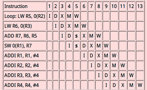Loop-unrooling 後的編譯流程圖： * 平均CPI = 16 clock cycles / 12 instuctions = 1.333. * 最終值計算出來後所需的CPI = 1.333 * 500 = 666.67 * 提升了接近3倍的效能 ![](https://hackpad-attachments.s3.amazonaws.com/embedded2016.hackpad.com_f5CCUGMQ4Kp_p.580980_1462022697807_2016-04-30%2021-13-02%20%E7%9A%84%E8%9E%A2%E5%B9%95%E6%93%B7%E5%9C%96.png) 從上述例子中，我們耶可以推論出： 1.Loop-unrooling 計算的陣列越大，Loop-unrooling 的效能提升會線性增長。(並非直接以*2計算效能增長) 2.但現實中許多例子都需考慮hazard的影響，如下圖： ![](https://hackpad-attachments.s3.amazonaws.com/embedded2016.hackpad.com_f5CCUGMQ4Kp_p.580980_1462023491931_2016-04-30%2021-37-39%20%E7%9A%84%E8%9E%A2%E5%B9%95%E6%93%B7%E5%9C%96.png) * 在這個例子中，當利用 Loop-unrooling 的運算式越來越複雜時，編譯器在遇到hazard時，需要等待前一個有hazard的變數解碼後才能執行下一行指令。 * 這說明了在有hazard時，運算式的複雜度越高，使用 Loop-unrooling 的效能提升越低。 3.在沒有hazard的情況下，Loop-unrooling 越多效能越高，但是在有hazard的情況下，Loop-unrooling 所提升的效能將會圖形將會呈現類似常態分佈的曲線圖，即會擁有最佳的 Loop-unrooling 數 * 可是該如何解釋在電腦上出現的效能結果呢？以add_vector( )爲例子：add_vector並沒有管線危害由： static inline void add_vector(const double *a, const double b, double *out) { for (int i = 0; i < 3; i++) out[i] = a[i] + b[i]; } 展開爲 static inline void add_vector(const double *a, const double b, double *out) { out[0] = a[0] + b[0]; out[1] = a[1] + b[1]; out[2] = a[2] + b[2]; } Loop-unrooling 後的組合語言應爲(我查不到ubuntu15.10所使用的組譯器，所以先使用DLX代替)： Loop: LW R5, 0(R2) ; element of b LW R6, 0(R3) ; element of c ADD R7, R6, R5 ; make out[0] LW R5, 4(R2) ; next element of b LW R6, 4(R3) ; next element of c ADD R8, R5, R6 ; make out[1] LW R5, 8(R2) ; next element of b LW R6, 8(R3) ; next element of c ADD R9, R5, R6 ; make out[2] SW 0(R1), R7 ; SW 4(R1), R8 ; SW 8(R1),R9 ; 由於沒有for迴圈，指令(instruction)數量爲12 * Loop-unrooling 前的CPI爲1.625 * 3 = 4.875 * Loop-unrooling 後的CPI爲16/12 = 1.333 * 提升效能應爲4.875 / 1.333 = 3.62625倍 * 通過執行兩個raytracing並查看gprof中add_vector的self_seconds的執行時間（因爲每一次執行時間都不一樣，所以通過執行十次並取其常態分佈）： * 結果爲： * Loop-unrooling 前的add_vector的常態執行時間爲0.22（最低0.15，最高0.25） * Loop-unrooling 後的add_vector的常態執行時間爲0.10（最低0.04，最高0.13） * 實際效能大約提高了2.2倍 * 每一次使用gprof查看執行時間都不一樣，雖取其常態分佈，但是實際提升效能與計算的不太一樣，不知是否計算結果錯誤，或是執行結果跳動幅度太大使實驗結果出錯.。會想辦法在gprof中利用類似hw1的phonebook程式中大量執行次數結果來進行驗證。 * 把add_vector function單獨執行，把實際增加效益與理論效益比較利用gcc的功能查看程式碼的組合語言：程式碼`： * #include <stdio.h> void loop(int *a,int *b,int *c) { for(int i = 0; i < 3;i++){ a[i] = b[i] + c[i]; } } int main() { int a[3] = {1}; int b[3] = {2}; int c[3] = {3}; loop(a,b,c); return 0; } 利用gcc -O0 -c test_loop_unrooling1.c 產生.o檔，再利用objdump -d test_loop_unrooling1.o查看組合語言 Loop 函式在-O0模式下的結果爲： 0000000000000000 <loop>: 0: 55 push %rbp 1: 48 89 e5 mov %rsp,%rbp 4: 48 89 7d e8 mov %rdi,-0x18(%rbp) 8: 48 89 75 e0 mov %rsi,-0x20(%rbp) c: 48 89 55 d8 mov %rdx,-0x28(%rbp) 10: c7 45 fc 00 00 00 00 movl $0x0,-0x4(%rbp) 17: eb 4a jmp 63 <loop+0x63> 19: 8b 45 fc mov -0x4(%rbp),%eax 1c: 48 98 cltq 1e: 48 8d 14 85 00 00 00 lea 0x0(,%rax,4),%rdx 25: 00 26: 48 8b 45 e8 mov -0x18(%rbp),%rax 2a: 48 01 d0 add %rdx,%rax 2d: 8b 55 fc mov -0x4(%rbp),%edx 30: 48 63 d2 movslq %edx,%rdx 33: 48 8d 0c 95 00 00 00 lea 0x0(,%rdx,4),%rcx 3a: 00 3b: 48 8b 55 e0 mov -0x20(%rbp),%rdx 3f: 48 01 ca add %rcx,%rdx 42: 8b 0a mov (%rdx),%ecx 44: 8b 55 fc mov -0x4(%rbp),%edx 47: 48 63 d2 movslq %edx,%rdx 4a: 48 8d 34 95 00 00 00 lea 0x0(,%rdx,4),%rsi 51: 00 52: 48 8b 55 d8 mov -0x28(%rbp),%rdx 56: 48 01 f2 add %rsi,%rdx 59: 8b 12 mov (%rdx),%edx 5b: 01 ca add %ecx,%edx 5d: 89 10 mov %edx,(%rax) 5f: 83 45 fc 01 addl $0x1,-0x4(%rbp) 63: 83 7d fc 02 cmpl $0x2,-0x4(%rbp) 67: 7e b0 jle 19 <loop+0x19> 69: 90 nop 6a: 5d pop %rbp 6b: c3 retq 在-O0的模式下編譯器所產生的組合語言把算式展開成3份，不論是多少層的迴圈數 Loop 函式在-O1和-O2模式下的結果爲： -O1 和 -O2模式中，loop函式並沒有被優化，而是針對main函式進行優化。 0000000000000000 <loop>: 0: b8 00 00 00 00 mov $0x0,%eax 5: 8b 0c 02 mov (%rdx,%rax,1),%ecx 8: 03 0c 06 add (%rsi,%rax,1),%ecx b: 89 0c 07 mov %ecx,(%rdi,%rax,1) e: 48 83 c0 04 add $0x4,%rax 12: 48 83 f8 0c cmp $0xc,%rax 16: 75 ed jne 5 <loop+0x5> 18: f3 c3 repz retq 把程式碼改成： #include <stdio.h> void loop(int *a,int *b,int *c) { a[0] = b[0] + c[0]; a[1] = b[1] + c[1]; a[2] = b[2] + c[2]; } int main() { int a[3] = {1}; int b[3] = {2}; int c[3] = {3}; loop(a,b,c); return 0; } -O0產生之組合語言爲： 0000000000000000 <loop>: 0: 55 push %rbp 1: 48 89 e5 mov %rsp,%rbp 4: 48 89 7d f8 mov %rdi,-0x8(%rbp) 8: 48 89 75 f0 mov %rsi,-0x10(%rbp) c: 48 89 55 e8 mov %rdx,-0x18(%rbp) 10: 48 8b 45 f0 mov -0x10(%rbp),%rax 14: 8b 10 mov (%rax),%edx 16: 48 8b 45 e8 mov -0x18(%rbp),%rax 1a: 8b 00 mov (%rax),%eax 1c: 01 c2 add %eax,%edx 1e: 48 8b 45 f8 mov -0x8(%rbp),%rax 22: 89 10 mov %edx,(%rax) 24: 48 8b 45 f8 mov -0x8(%rbp),%rax 28: 48 83 c0 04 add $0x4,%rax 2c: 48 8b 55 f0 mov -0x10(%rbp),%rdx 30: 48 83 c2 04 add $0x4,%rdx 34: 8b 0a mov (%rdx),%ecx 36: 48 8b 55 e8 mov -0x18(%rbp),%rdx 3a: 48 83 c2 04 add $0x4,%rdx 3e: 8b 12 mov (%rdx),%edx 40: 01 ca add %ecx,%edx 42: 89 10 mov %edx,(%rax) 44: 48 8b 45 f8 mov -0x8(%rbp),%rax 48: 48 83 c0 08 add $0x8,%rax 4c: 48 8b 55 f0 mov -0x10(%rbp),%rdx 50: 48 83 c2 08 add $0x8,%rdx 54: 8b 0a mov (%rdx),%ecx 56: 48 8b 55 e8 mov -0x18(%rbp),%rdx 5a: 48 83 c2 08 add $0x8,%rdx 5e: 8b 12 mov (%rdx),%edx 60: 01 ca add %ecx,%edx 62: 89 10 mov %edx,(%rax) 64: 90 nop 65: 5d pop %rbp 66: c3 retq - -O1產生之組合語言爲： 0000000000000000 <loop>: 0: 8b 02 mov (%rdx),%eax 2: 03 06 add (%rsi),%eax 4: 89 07 mov %eax,(%rdi) 6: 8b 42 04 mov 0x4(%rdx),%eax 9: 03 46 04 add 0x4(%rsi),%eax c: 89 47 04 mov %eax,0x4(%rdi) f: 8b 42 08 mov 0x8(%rdx),%eax 12: 03 46 08 add 0x8(%rsi),%eax 15: 89 47 08 mov %eax,0x8(%rdi) 18: c3 retq **Force Inline** * references： * [深入理解内联inline函数的优缺点，性能及使用指南](http://blog.csdn.net/acs713/article/details/42649949) * [Extern Vs Static Inline](http://elinux.org/Extern_Vs_Static_Inline) * [Inline Functions In C](http://www.greenend.org.uk/rjk/tech/inline.html) * [C/C++中inline/static inline/extern inline的区别及使用](http://blog.csdn.net/fengbingchun/article/details/51234209) * inline是向編譯器提出“建議”，把inline的函數在函數位置直接展開（減輕系統負擔(overhead)），編譯器會對比兩者執行時間後選擇執行inline與否。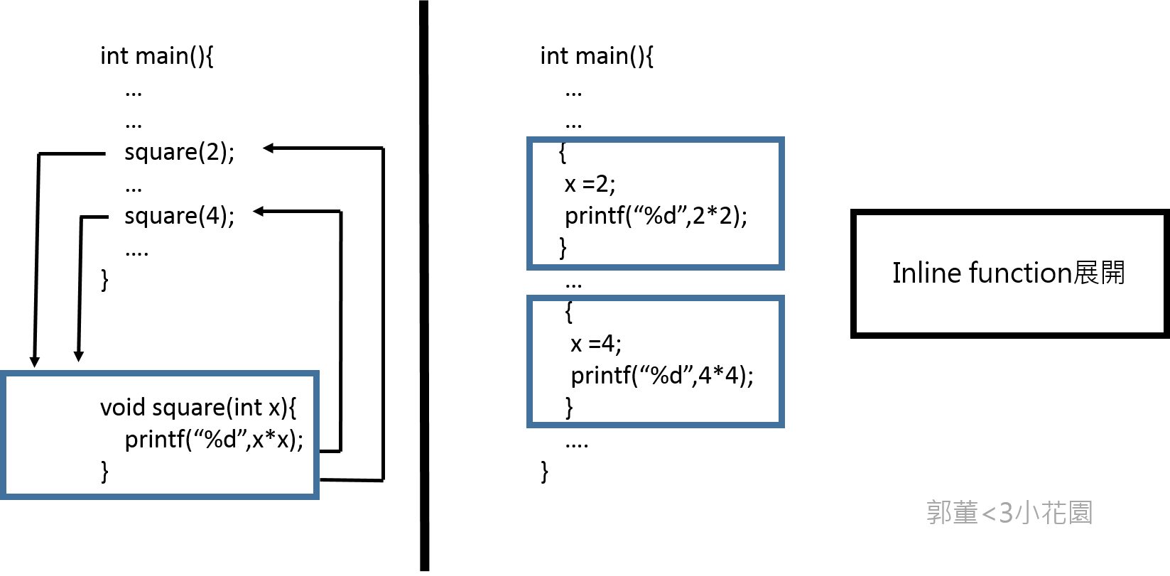 * 使用inline能夠減少2億次的function call ![](https://hackpad-attachments.s3.amazonaws.com/embedded2016.hackpad.com_f5CCUGMQ4Kp_p.580980_1462031288192_20131127195935156.png) * 因爲在Makefile中擁有 -O0 的指令（關閉最佳化），所以inline不會被執行，要讓inline執行必須在每一個function後面加上__attribute__((always_inline))強行讓CPU去執行inline這個“建議” * force_inline後的執行時間： #Rendering scene Done! Execution time of raytracing() : 3.730698 sec 在gprof中可以看到，被強制inline的function已經追蹤不到了，因爲他們已被展開 Each sample counts as 0.01 seconds. % cumulative self self total time seconds seconds calls s/call s/call name 33.11 0.95 0.95 13861875 0.00 0.00 rayRectangularIntersection 26.84 1.72 0.77 13861875 0.00 0.00 raySphereIntersection 12.20 2.07 0.35 2110576 0.00 0.00 compute_specular_diffuse 7.32 2.28 0.21 1048576 0.00 0.00 ray_color 6.27 2.46 0.18 1048576 0.00 0.00 rayConstruction 4.53 2.59 0.13 2110576 0.00 0.00 localColor 4.18 2.71 0.12 4620625 0.00 0.00 ray_hit_object 1.39 2.75 0.04 1241598 0.00 0.00 refraction 1.05 2.78 0.03 2520791 0.00 0.00 idx_stack_top 1.05 2.81 0.03 1241598 0.00 0.00 protect_color_overflow 1.05 2.84 0.03 1241598 0.00 0.00 reflection 0.70 2.86 0.02 1 0.02 2.87 raytracing 0.17 2.87 0.01 1204003 0.00 0.00 idx_stack_push 0.17 2.87 0.01 1048576 0.00 0.00 idx_stack_init 0.00 2.87 0.00 2558386 0.00 0.00 idx_stack_empty 0.00 2.87 0.00 113297 0.00 0.00 fresnel 0.00 2.87 0.00 37595 0.00 0.00 idx_stack_pop 0.00 2.87 0.00 3 0.00 0.00 append_rectangular 0.00 2.87 0.00 3 0.00 0.00 append_sphere 0.00 2.87 0.00 2 0.00 0.00 append_light 0.00 2.87 0.00 1 0.00 0.00 calculateBasisVectors 0.00 2.87 0.00 1 0.00 0.00 delete_light_list 0.00 2.87 0.00 1 0.00 0.00 delete_rectangular_list 0.00 2.87 0.00 1 0.00 0.00 delete_sphere_list 0.00 2.87 0.00 1 0.00 0.00 diff_in_second 0.00 2.87 0.00 1 0.00 0.00 write_to_ppm Inline優缺點、效能與使用指南： * 優點： * 減輕系統負擔，呼叫函式或返回值時。 * 利用指令的緩存提高**locality of reference（參考局部性）** * 問：爲什麼會提高參考局部性？ * instruction cache ! 回去讀書 * Keyword: The Locality Principle : [](https://www.cs.utexas.edu/~fussell/courses/cs429h/lectures/Lecture_18-429h.pdf)https://www.cs.utexas.edu/~fussell/courses/cs429h/lectures/Lecture_18-429h.pdf * [](https://www.cs.umd.edu/class/fall2001/cmsc411/proj01/cache/matrix.html)https://www.cs.umd.edu/class/fall2001/cmsc411/proj01/cache/matrix.html * 使用inline後也能使用 intraprocedural optmization(程序間優化) 。讓編譯器能夠專注在其他方面。例如：dead code elimination、branch predictionif specified. induction variable elimination。 * Interprocedural optimization (IPO) 爲ICC(intel C++ compiler)編譯器提供的技術 (gcc 也有實做)，打破了傳統編譯器只把優化過程注重在原始程式碼檔案內部，不注重在鏈接過程中的優化。傳統優化過程中在優化都是獨立進行的。IPO 在編譯時產生一個新的語言(中間語言)，在連結和編譯時都進行優化。如下圖： ![](https://hackpad-attachments.s3.amazonaws.com/embedded2016.hackpad.com_f5CCUGMQ4Kp_p.580980_1462045772267_ipo.png) * 詳細的優化項目課參考intel網站：[Interprocedural Optimization (IPO)](https://software.intel.com/en-us/node/522667) * [icc的過程間優化和性能分析引導優化](https://www.byvoid.com/blog/icc-ipo-pgo) * 缺點： * 造成程式過於龐大，增加cache miss、減少可讀性、造成編譯器和記憶體的負擔 * 嵌入後的函式如涉及變數在暫存器的存取，會對系統造成很大的負擔 * 造成編譯器的負擔可讀性大大減少(程式碼太多) * <s>以嵌入式設計而言，嵌入函式是非常沒有用（嵌入式的程式以簡短爲主）</s> * 過於武斷，嵌入式系統不表示「小系統」 * 使用指南： * 確定效能的提高後才使用 * 不要以巨集代替 inline function * 不要展開過於龐大的程式碼 inline、static Inline與 extern inline的差別： * 在elinux wiki中有一句話： - "static inline" means "we have to have this function, if you use it but don’t inline it, then make a static version of it in this compilation unit" - "extern inline" means "I actually _have_ an extern for this function,but if you want to inline it, here’s the inline-version" - ... we should just convert all current users of "extern inline" to "static inline". - static inline是直接把該段函式直接展開被呼叫的地方，所以它並不會產生函式程式碼 - inline與static inline相同只是函式本身可能還會被會被其他編譯單元呼叫，所以在原有處會產生代碼 - extern inline(也可以用macro代替)與extern的用意類似，都是告訴編譯器函式可以被多次定義。防止多次宣告導致編譯器建立多個地址去儲存相同的函式或浪費記憶題空間 * 用法： * extern inline除了直接宣告，也可以利用macro： #ifndef INLINE #define INLINE extern inline #endif INLINE int max(int a, int b) { return a > b ? a : b; } * 實作可移植性高的inline函式： #ifndef INLINE #if __GNUC__ && !__GNUC_STDC_INLINE__ # define INLINE extern inline #else # define INLINE inline #endif #endif INLINE int max(int a, int b) { return a > b ? a : b; } //...and in exactly one source file: #define INLINE #include "header.h" * 不是很明白上述巨集的使用方式，是否讓編譯器自己決定使用哪一種方式進行優化？ * gcc -O0 (關閉最佳化) 的時候，"inline" 關鍵字是沒有效果的，連帶 INLINE 不會有作用，所以上述技巧可在編譯時期知曉程式輸出 **MACRO** * references： * [Macros ](https://gcc.gnu.org/onlinedocs/cpp/index.html#Top) * [前置處理器](http://epaper.gotop.com.tw/pdf/ael005600.pdf) 巨集在編譯之前（前置處理）就已經被代換成指定的表示法或數值 * 方法：把dot_product利用巨集的方法定義即： * #define dot_product(a,b) ((a[0]*b[0])+(a[1]*b[1])+(a[2]*b[2])) 執行結果爲： #Rendering scene Done! Execution time of raytracing() : 5.518978 sec - 而只inline dot_product( )的執行時間結果爲： #Rendering scene Done! Execution time of raytracing() : 6.447092 sec macro的效能提升比inline多了大約1.168倍(0.9sec) * 提升這麼多是基於dot_product將近700萬次的呼叫次數 * Macro與inline function的比較： * references： * [Inline function、Marco](http://ascii-iicsa.blogspot.tw/2010/08/inline-functionmarco.html) * [Inline functions vs Preprocessor macros](http://stackoverflow.com/questions/1137575/inline-functions-vs-preprocessor-macros) * [Why are preprocessor macros evil and what are the alternatives](http://stackoverflow.com/questions/14041453/why-are-preprocessor-macros-evil-and-what-are-the-alternatives) * 兩個在功能上非常接近，但是<s>巨集不能被編譯器debug</s> * 問：什麼意思不能被編譯器debug？ * 這說法不對！只要編譯器設計夠好，還是能對巨集進行除錯分析: * [](https://gcc.gnu.org/onlinedocs/gcc/Debugging-Options.html)https://gcc.gnu.org/onlinedocs/gcc/Debugging-Options.html # 注意看 `-g3` 的用法 * 交叉對照 force inline * gcc要加tag就可以debug 巨集拉看一下hw2共筆的參考資料 * <s>巨集在使用彈性方面比內嵌函式大</s> * 說法不精確！修正 * <u>以下是Macro跟call function的優缺點：</u> * 巨集　(macro) * 優點：執行速度快，沒有堆疊的 push 和 pop 動作的需要，減少時間的耗損。 * 缺點：巨集被呼叫多次以後，會耗損存放及使用大量的記憶體空間。 * 函數　(call function/call subroutine) * 優點：即使函數被呼叫多次，在記憶體中仍只有一份實體，較節省記憶體空間。能節省存放及使用的記憶體空間。 * 缺點：執行速度較慢，需花費時間在堆疊的 push 和 pop 動作上。 * 結論：在使用巨集作爲函式時需非常小心(命名、結構方面)，不然結果將會是錯誤的且編譯器不能幫你偵測和分析，但是它的效能的比較上比inline function效果好些，忽略記憶體空間來說的話。 **SIMD** * references：[](https://www.youtube.com/watch?v=s6SXj3v-a38)[https://www.youtube.com/watch?v=s6SXj3v-a38](https://www.youtube.com/watch?v=s6SXj3v-a38) [](http://www.codeproject.com/Articles/874396/Crunching-Numbers-with-AVX-and-AVX)[http://www.codeproject.co](http://www.codeproject.co/)[m/Articles/874396/Crunching-Numbers-with-AVX-and-AVX](http://www.codeproject.co%20m/Articles/874396/Crunching-Numbers-with-AVX-and-AVX) [](https://software.intel.com/sites/landingpage/IntrinsicsGuide/#expand=2932,3559,3580,3632,3900,4574,4578,5474,5472,5471,5616,5661,5670,5692,5693,560,563,585,687,1680,2928,2930&techs=AVX)https://software.intel.com/sites/landingpage/IntrinsicsGuide/#expand=2932,3559,3580,3632,3900,4574,4578,5474,5472,5471,5616,5661,5670,5692,5693,560,563,585,687,1680,2928,2930&techs=AVX avx是sse指令集的一種支援的bit比sse sse2..等等還多下表是avx的資料型態 <table style="color: rgb(0, 0, 0); font-family: Helvetica; letter-spacing: normal; font-size: 13px;"> <tbody> <tr> <td class="added" style="border: 1px solid rgb(153, 153, 153); min-width: 50px; height: 22px; line-height: 16px; padding-right: 4px; padding-left: 4px;">Data Type</td> <td class="added" style="border: 1px solid rgb(153, 153, 153); min-width: 50px; height: 22px; line-height: 16px; padding-right: 4px; padding-left: 4px;">Description</td> </tr> <tr> <td class="added" style="border: 1px solid rgb(153, 153, 153); min-width: 50px; height: 22px; line-height: 16px; padding-right: 4px; padding-left: 4px;">__m128</td> <td class="added" style="border: 1px solid rgb(153, 153, 153); min-width: 50px; height: 22px; line-height: 16px; padding-right: 4px; padding-left: 4px;">128-bit vector containing 4 floats</td> </tr> <tr> <td class="added" style="border: 1px solid rgb(153, 153, 153); min-width: 50px; height: 22px; line-height: 16px; padding-right: 4px; padding-left: 4px;">__m128d</td> <td class="added" style="border: 1px solid rgb(153, 153, 153); min-width: 50px; height: 22px; line-height: 16px; padding-right: 4px; padding-left: 4px;">128-bit vector containing 2 doubles</td> </tr> <tr> <td class="added" style="border: 1px solid rgb(153, 153, 153); min-width: 50px; height: 22px; line-height: 16px; padding-right: 4px; padding-left: 4px;">__m128i</td> <td class="added" style="border: 1px solid rgb(153, 153, 153); min-width: 50px; height: 22px; line-height: 16px; padding-right: 4px; padding-left: 4px;">128-bit vector containing integers</td> </tr> <tr> <td class="added" style="border: 1px solid rgb(153, 153, 153); min-width: 50px; height: 22px; line-height: 16px; padding-right: 4px; padding-left: 4px;">__m256</td> <td class="added" style="border: 1px solid rgb(153, 153, 153); min-width: 50px; height: 22px; line-height: 16px; padding-right: 4px; padding-left: 4px;">256-bit vector containing 8 floats</td> </tr> <tr> <td class="added" style="border: 1px solid rgb(153, 153, 153); min-width: 50px; height: 22px; line-height: 16px; padding-right: 4px; padding-left: 4px;">__m256d</td> <td class="added" style="border: 1px solid rgb(153, 153, 153); min-width: 50px; height: 22px; line-height: 16px; padding-right: 4px; padding-left: 4px;">256-bit vector containing 4 doubles</td> </tr> <tr> <td class="added" style="border: 1px solid rgb(153, 153, 153); min-width: 50px; height: 22px; line-height: 16px; padding-right: 4px; padding-left: 4px;">__m256i</td> <td class="added" style="border: 1px solid rgb(153, 153, 153); min-width: 50px; height: 22px; line-height: 16px; padding-right: 4px; padding-left: 4px;">256-bit vector containing integers</td> </tr> </tbody> </table> 因為內積函數一次要將三個64bit相乘需要3*64 ＝ 192 bit 所以必須使用avx指令集想在intel上使用avx指令集，要在cflag 加 -mavx2 ，並加入#include<immintrin.h> * 在使用simd之前，程式的執行時間大約都在2.05秒左右 * 這時候把dot_product函數從 * _<u> return v1[0]*v2[0]+v1[1]*v2[1]+v1[2]*v2[2]; </u>_ * 更改成 double dp[4]; __m256d v_1 = _mm256_loadu_pd(v1); __m256d v_2 = _mm256_loadu_pd(v2); _mm_prefetch((const char*)(v1), _MM_HINT_NTA); _mm_prefetch((const char*)(v2), _MM_HINT_NTA); __m256d mul = _mm256_mul_pd(v_1, v_2); _mm256_storeu_pd(dp,mul); return (dp[0] + dp[1] + dp[2]); * 結果時間暴衝了兩倍多變成4.6秒 __m256d vv1 = _mm256_set_pd(0,v1[2],v1[1],v1[0]); __m256d vv2 = _mm256_set_pd(0,v2[2],v2[1],v2[0]); __m256d v1v2 = _mm256_mul_pd(vv1,vv2); return (v1v2[0]+v1v2[1]+v1v2[2]); 這個版本時間平均為3.4秒 double tmp[4] __attribute__((aligned(32))); __m256d x = _mm256_set_pd( v1[0], v1[1], v1[2], 0.0); __m256d y = _mm256_set_pd( v2[0], v2[1], v2[2], 0.0); __m256d xy = _mm256_mul_pd(x, y); _mm256_store_pd(tmp, xy); return (tmp[0] + tmp[1] + tmp[2] + tmp[3]); 這個版本時間平均為3.6秒可以看出第二個版本因為沒有用tmp另外存一次所以速度比較快但還是比不用simd還慢使用simd的時候要讓資料對齊對齊與否會影響速度原因如下, _ Because accessing memory on an address that is not divisible by the bus size takes a lot of transistors. x86 and x64 cores can do it with zero cycle overhead for values up to the native register size (32 or 64 bits)_ 在dot product使用simd時,根據上面第二份code 1最初的v1 v2 loading大概需要4*2次,加上_mm256_mul_pd 1次,最後的return loading 3次 +了2次 ,總共是14次而改成simd前的code只要loading6次+2次*3次,總共只有11次本來simd需要的指令就比較多，又加上simd版本的loading指令較多（loading會比算術運算更耗時間），所以在dot product使用simd一定會比原來的慢 * 這結論不精確！ * 仍可進一步調整: [SIMD Ray Tracing Tips](http://graphics.ucsd.edu/courses/cse168_s10/ucsd/SIMD_Ray_Tracing_Tips.pdf); [Real-Time Ray Tracing](http://www.cs.cmu.edu/afs/cs/academic/class/15869-f11/www/lectures/14_raytracing.pdf); * => [](http://www.joshbarczak.com/blog/?p=787)http://www.joshbarczak.com/blog/?p=787 * 這個解釋對於dotproduct是對的。閱讀資料後進一步修改結論 **OpenMP** * references： * [OpenMP简易教程(pdf)](https://drive.google.com/open?id=0B4WZ6ihm_C7zYkdvNUJyYlJFRG8) * [Sun Studio 12 Update 1：OpenMP API 用户指南](https://docs.oracle.com/cd/E19205-01/821-0393/6nletfa30/index.html) * [Common Mistakes in OpenMP and How To Avoid Them](http://michaelsuess.net/publications/suess_leopold_common_mistakes_06.pdf) * **OpenMP**（Open Multi-Processing）是一套支持跨平台、共享記憶體方式的多執行緒平行運算的API。 * 它比起使用作業系統直接建立執行緒有三大優點： * CPU核心數量的擴展性 * 便利性 * 可移植性 * 以下爲OpenMP在光影追蹤程式碼中的用法： * #pragma omp parallel for schedule(guided,1) collapse(2) num_threads(64) private(stk), private(d),private(object_color) * OpenMP的呼叫需 `#include<omp.h>` 及在編譯時加入-fopenmp -lgomp指令 * OpenMP的用法： * 平行設計 * parallel：用以建造一個平行塊 * 資料處理 * 資料處理在OpenMP是最爲重要的一部分，例如private( )：它把變數宣告爲私有變數，讓其他執行緒無法存取，可以解決race condition的問題。 * 任務排程 * schedule：有四種類型：dynamic、guided、runtime和static，使用時可以根據程式的結構對線程進行不同調度。 * 使用private( )對stk、d和object_color進行處理的原因 * 在迴圈中的變數有非常多，但是可以從程式碼中看到以下兩行，<s>他們的值事先就已經好</s> (這是中文嗎？)，他們的值在進入迴圈之前就已進行過一次運算，並且在迴圈內並沒有任何一行指令會去改變他們的值，所以可想而知它們的值是不會改變的。所以只剩下stk、d和object_color這三個變數了。 * calculateBasisVectors(u, v, w, view); * int factor = sqrt(SAMPLES); * 利用對迴圈內運算結果的輸出證明： - #Rendering scene ```shell= u =-0.707107,0.707107,0.000000 v =-0.408248,-0.408248,0.816497 w = -0.577350,-0.577350,-0.577350 d = -7.594374,-15.545776,-4.683959 u =-0.707107,0.707107,0.000000 v =-0.408248,-0.408248,0.816497 w = -0.577350,-0.577350,-0.577350 d = -0.423520,-0.867212,-0.261868 u =-0.707107,0.707107,0.000000 v =-0.408248,-0.408248,0.816497 w = -0.577350,-0.577350,-0.577350 d = -0.424204,-0.867028,-0.261367 u =-0.707107,0.707107,0.000000 v =-0.408248,-0.408248,0.816497 w = -0.577350,-0.577350,-0.577350 d = -0.424035,-0.866945,-0.261918 u =-0.707107,0.707107,0.000000 v =-0.408248,-0.408248,0.816497 w = -0.577350,-0.577350,-0.577350 d = -0.424719,-0.866761,-0.261417 u =-0.707107,0.707107,0.000000 v =-0.408248,-0.408248,0.816497 w = -0.577350,-0.577350,-0.577350 d = -0.424550,-0.866677,-0.261969 u =-0.707107,0.707107,0.000000 v =-0.408248,-0.408248,0.816497 w = -0.577350,-0.577350,-0.577350 d = -0.425234,-0.866493,-0.261468 u =-0.707107,0.707107,0.000000 v =-0.408248,-0.408248,0.816497 w = -0.577350,-0.577350,-0.577350 d = -0.425065,-0.866410,-0.262019 u =-0.707107,0.707107,0.000000 v =-0.408248,-0.408248,0.816497 w = -0.577350,-0.577350,-0.577350 d = -0.425749,-0.866225,-0.261518 u =-0.707107,0.707107,0.000000 ``` 在沒有設定private的情況下，可以發現 u、v、w的值是固定的，而d的值是以遞減的狀態改變的。當使用多執行緒時，若沒有把d的值宣告爲私有變數，那麼就會出現race conditon的情況(因爲多執行緒並不會按順序進行工作) 而在設定private(w || u || v)的情況下，他們輸出結果爲0，說明了private的變數不會讀取之前運算的值。 * OpenMP在什麼情況下可提升效能？ * OpenMP在處理並行工作時是使用平均分配的方法，以光影追蹤爲例，產生的圖片每個地方的複雜度是不一樣的，如果依照平均分配工作要進行任務，被分派至複雜度高區域做工的執行緒會比其他的慢。 * 所以OpenMP比較適合在執行工作複雜度叫平均的程式碼上 * OpenMP執行速度： #Rendering scene Done! Execution time of raytracing() : 1.657689 sec 利用組合語言觀察private的實作並解釋 - Private的操作原理 references：\[汇编lea 指令与 mov 指令\](http://blog.sina.com.cn/s/blog_4c4d6e7401016kdk.html) 利用程式產生值組合語言理解private實際操作原理：程式： ```clike= #include<stdio.h> #include<omp.h> int main(){ int a = 0; #pragma omp parallel for // + private(a) for(int i=0; i < 5;i++){ a = a + 5; } } ``` 以下爲沒有private時的組合語言： * 0000000000000060 <main.\_omp\_fn.0>: 60: 55 push %rbp 61: 48 89 e5 mov %rsp,%rbp 64: 53 push %rbx 65: 48 83 ec 28 sub $0x28,%rsp 69: 48 89 7d d8 mov %rdi,-0x28(%rbp) 6d: c7 45 ec 00 00 00 00 movl $0x0,-0x14(%rbp) 74: e8 00 00 00 00 callq 79 <main.\_omp\_fn.0+0x19> 79: 89 c3 mov %eax,%ebx 7b: e8 00 00 00 00 callq 80 <main.\_omp\_fn.0+0x20> 80: 89 c6 mov %eax,%esi 82: b8 05 00 00 00 mov $0x5,%eax 87: 99 cltd 88: f7 fb idiv %ebx 8a: 89 c1 mov %eax,%ecx 8c: b8 05 00 00 00 mov $0x5,%eax 91: 99 cltd 92: f7 fb idiv %ebx 94: 89 d0 mov %edx,%eax 96: 39 c6 cmp %eax,%esi 98: 7c 2b jl c5 <main.\_omp\_fn.0+0x65> 9a: 0f af f1 imul %ecx,%esi 9d: 89 f2 mov %esi,%edx 9f: 01 d0 add %edx,%eax a1: 8d 14 08 lea (%rax,%rcx,1),%edx a4: 39 d0 cmp %edx,%eax a6: 7d 27 jge cf <main.\_omp\_fn.0+0x6f> a8: 89 45 ec mov %eax,-0x14(%rbp) ab: 48 8b 45 d8 mov -0x28(%rbp),%rax af: 8b 00 mov (%rax),%eax b1: 8d 48 05 lea 0x5(%rax),%ecx b4: 48 8b 45 d8 mov -0x28(%rbp),%rax b8: 89 08 mov %ecx,(%rax) ba: 83 45 ec 01 addl $0x1,-0x14(%rbp) be: 39 55 ec cmp %edx,-0x14(%rbp) c1: 7c e8 jl ab <main.\_omp\_fn.0+0x4b> c3: eb 0a jmp cf <main.\_omp\_fn.0+0x6f> c5: b8 00 00 00 00 mov $0x0,%eax ca: 83 c1 01 add $0x1,%ecx cd: eb cb jmp 9a <main.\_omp\_fn.0+0x3a> cf: 48 83 c4 28 add $0x28,%rsp d3: 5b pop %rbx d4: 5d pop %rbp d5: c3 retq 以下爲有private時的組合語言： * 000000000000002f <main.\_omp\_fn.0>: 2f: 55 push %rbp 30: 48 89 e5 mov %rsp,%rbp 33: 53 push %rbx 34: 48 83 ec 28 sub $0x28,%rsp 38: 48 89 7d d8 mov %rdi,-0x28(%rbp) 3c: c7 45 e8 00 00 00 00 movl $0x0,-0x18(%rbp) 43: e8 00 00 00 00 callq 48 <main.\_omp\_fn.0+0x19> 48: 89 c3 mov %eax,%ebx 4a: e8 00 00 00 00 callq 4f <main.\_omp\_fn.0+0x20> 4f: 89 c6 mov %eax,%esi 51: b8 05 00 00 00 mov $0x5,%eax 56: 99 cltd 57: f7 fb idiv %ebx 59: 89 c1 mov %eax,%ecx 5b: b8 05 00 00 00 mov $0x5,%eax 60: 99 cltd 61: f7 fb idiv %ebx 63: 89 d0 mov %edx,%eax 65: 39 c6 cmp %eax,%esi 67: 7c 20 jl 89 <main.\_omp\_fn.0+0x5a> 69: 0f af f1 imul %ecx,%esi 6c: 89 f2 mov %esi,%edx 6e: 01 d0 add %edx,%eax 70: 8d 14 08 lea (%rax,%rcx,1),%edx 73: 39 d0 cmp %edx,%eax 75: 7d 1c jge 93 <main.\_omp\_fn.0+0x64> 77: 89 45 e8 mov %eax,-0x18(%rbp) 7a: 83 45 ec 05 addl $0x5,-0x14(%rbp) 7e: 83 45 e8 01 addl $0x1,-0x18(%rbp) 82: 39 55 e8 cmp %edx,-0x18(%rbp) 85: 7c f3 jl 7a <main.\_omp\_fn.0+0x4b> 87: eb 0a jmp 93 <main.\_omp\_fn.0+0x64> 89: b8 00 00 00 00 mov $0x0,%eax 8e: 83 c1 01 add $0x1,%ecx 91: eb d6 jmp 69 <main.\_omp\_fn.0+0x3a> 93: 48 83 c4 28 add $0x28,%rsp 97: 5b pop %rbx 98: 5d pop %rbp 99: c3 retq 兩段組合語言的差別在。。。。。。 * Hint: tls (thread local storage) **消除 assert 對效能的影響** * 方法：修改 Makefile，新增 \`CFLAGS=-DNDEBUG\` 以消除 assert 對效能的影響，或是直接刪除assert的程式碼。 * assert( ) * 是一個診斷巨集，用於動態辨識程式的邏輯錯誤條件。原型爲： * void assert(int expression); * 如巨集的參數求值與assert不符，assert會輸出維護敘述並執行abort( )： * assert(d != 0.0 && "Error calculating normal"); * 在math-toolkit.h中的normalize( )判斷normalize的向量如果爲0則輸出字串並停止運行程式。 * 修改後的執行時間快了0.1秒 * 因爲執行normalize的次數高達1000萬次 * \# Rendering scene * Done! * Execution time of raytracing() : 3.242110 sec \[ 03:37 \] assert() 本質是個 macro，所以會仰賴 \`NDEBUG\` macro 的定義結果而有不同的行為。assert() 在執行時期的原理為何？ * references： * \[ERR06-C. Understand the termination behavior of assert() and abort()\](https://www.securecoding.cert.org/confluence/pages/viewpage.action?pageId=16450219) \*\*POSIX Thread\*\* <u>多核心程式的好處：</u> * Parallelism：一個系統可以同時執行多個任務 * Data Parallelism：分佈相同的資料子集在多核心，每個資料具有相同的運作 * Task Parallelism：分佈執行緒在核心中，每個執行緒具有獨特的運作單核心系統： !\[\](https://hackpad-attachments.s3.amazonaws.com/embedded2016.hackpad.com\_f5CCUGMQ4Kp\_p.575390\_1462027662288\_QQ%E5%9B%BE%E7%89%8720140412155713.jpg) 多核心系統： !\[\](https://hackpad-attachments.s3.amazonaws.com/embedded2016.hackpad.com\_f5CCUGMQ4Kp\_p.575390\_1462027650685\_QQ%E5%9B%BE%E7%89%8720140412155722.jpg) 單執行緒和多執行緒的比較： !\[\](https://hackpad-attachments.s3.amazonaws.com/embedded2016.hackpad.com\_f5CCUGMQ4Kp\_p.575390\_1462027748751\_QQ%E5%9B%BE%E7%89%8720140412161344.jpg) 阿達爾定律（Amdahl’s Law）：實做多核心對程式效能的影響如何，又能夠提升多少效能提昇？設： * S：爲序列 (serial) 部分 * N：爲核心數量 !\[\](https://hackpad-attachments.s3.amazonaws.com/embedded2016.hackpad.com\_f5CCUGMQ4Kp\_p.575390\_1462051717109\_QQ%E5%9B%BE%E7%89%8720140412162050.jpg) 因此當我的核心是4（N），且程式序列執行部分爲5%（S），那麼我的程式會比原本的執行速度快接近3.5倍。當N趨近於無窮大時，speedup則趨近於 1/S，這表明了如果可以並行的部分不多，就算再多的核心，也不能增快程式的執行時間。以下會以實做來證明此定律。 PThread： PThread定義了一套C語言的型態定義、函數和常數。Pthread API中大致共有100個函式呼叫，全都以"pthread_"開頭，並可以分為四類： * 執行緒管理，例如建立執行緒、等待執行緒、查詢執行緒狀態等。 * Mutex：建立、銷毀、鎖定、解鎖、設定屬性等操作 * Condition Variable：建立、消滅、等待、通知、設定與查詢屬性等操作 * 使用了讀寫鎖的執行緒間的同步管理在使用pthread_create的時候，如果function的參數超過一個，那就必須把參數都包裝起來，利用指標傳入。如下： ```clike= /\* raytracing 中的所有參數 */ typedef struct __DATA { uint8_t *pixels; color background; rectangular_node rectangulars; sphere_node spheres; light_node lights; const viewpoint *View; int row; int col; int start\_j,end\_j; int start\_i,end\_i; point3 u, v, w, d; } arg_data; pthread\_create(&THREAD\[i\],NULL,(void*)raytracing,(void*)&arg\_data); ``` 參考資料：\[\](https://zh.wikipedia.org/wiki/POSIX%E7%BA%BF%E7%A8%8B)https://zh.wikipedia.org/wiki/POSIX%E7%BA%BF%E7%A8%8B 實做方面：利用Thread將圖片切割成不同的部分來實做，讓每個部分都可以並行處理，下是不同切割的想法： * 均分COL或ROW * 均分4個部分 * 上左、上右、下左、下右 * 根據每個部分複雜度不同而實做 * 可以降低每個thread的時間差，讓比較快做完的thread不必等慢的太久 * 比較複雜部分的先做 * 縮小比較複雜的部分，減少計算這個部分的執行緒的時間 <u>首先是實做均分COL：</u> ```clike= #MAX_THREAD=4 for(int i=0; i<MAX_THREAD; i++){ data\[i\].pixels = pixels; data\[i\].lights = lights; data\[i\].rectangulars = rectangulars; data\[i\].spheres = spheres; data\[i\].View = view; data\[i\].start_j = i; ptread_create(&THREAD\[i\],NULL,(void*)ray,(void*)&data\[i\]); if(pthread_create&THREAD\[i\],NULL,(void*)ray,(void*)&data\[i\])) { printf("ERROR thread create!\\n"); pthread_exit(NULL); } } for(int i=0; i<MAXX; i++) pthread_join(THREAD\[i\],NULL); for (int j = (*data).start\_j ; j < 512; j+=MAX\_THREAD) { for (int i = 0 ; i < 512; i++) { ``` ``` \# Rendering scene Done! Execution time of raytracing() : 1.636069 sec ``` <u>均分ROW：</u> for (int j = 0 ; j < 512; j++) { for (int i = (*data).start\_i ; i < 512; i+=MAX\_THREAD) { #Rendering scene Done! Execution time of raytracing() : 1.651790 sec <u>分成4個部分：</u> for(int i=0; i<MAX_THREAD; i++){ data\[i\].start_j = 256 - (256 * ((i+1)%2) ); data\[i\].end_j = 512 - ( 256 * ((i+1)%2) ); data\[i\].start_i = 0 + (256 * ((i+1)/3) ); data\[i\].end_i = 256 + ( 256 * ((i+1)/3) ); } for (int j = (\*data).start\_j ; j < (\*data).end\_j; j++) { for (int i = (\*data).start\_i ; i < (\*data).end\_i; i++) { #Rendering scene Done! Execution time of raytracing() : 1.681594 sec <u>根據複雜度不同而實做：</u> * 首先是需要計算出哪個部分是最複雜的，將每個部分的顏色都調整成同一個顏色，再利用一個變數記錄複雜度（顏色越深表示複雜度越高）： int complexity = 0; if (ray_color(view->vrp, 0.0, d, &stk, rectangulars, spheres, lights, object_color, MAX\_REFLECTION\_BOUNCES, &complexity)) /\* TMP 用來調整顏色比例 */ pixels\[((i + (j * width)) * 3) + 0\] = complexity * 255 / TMP; 結果圖如下： ![](https://hackpad-attachments.s3.amazonaws.com/embedded2016.hackpad.com\_f5CCUGMQ4Kp\_p.575390\_1462118230247\_out.png) 這樣就能確定哪個部分是最複雜的，這樣如果分配好每個thread的工作，那就能降低每個thread時間差的問題。 * 優化方式並不能針對所有情況，實作出能針對所有情況之方法 <u>縮小較複雜的部分：</u> - 讓其它thread幫忙分擔一點複雜的部分，好讓所有thread的執行時間都一致。 - 將所有thread個別指定數值（0~135，135~220，220~315，315~512）： data\[0\].pixels = pixels; data\[0\].lights = lights; data\[0\].rectangulars = rectangulars; data\[0\].spheres = spheres; data\[0\].View = view; data\[0\].start_i = 0; data\[0\].end_i = 135; pthread_create(&THREAD\[0\],NULL,(void*)ray,(void*)&data\[0\]); #Rendering scene Done! Execution time of raytracing() : 1.755379 sec 以上結果比較圖： ![](https://hackpad-attachments.s3.amazonaws.com/embedded2016.hackpad.com\_f5CCUGMQ4Kp\_p.575390\_1462124430461\_thread_runtime.png) <u>再來是Thread的數量：</u> * 理論上來說，Thread的數量多寡並不會影響到程式的效率，一切取決於處理器的核心，如果是 4核，那麼Thread的數量再多，程式的效率也跟4個（Thread）一樣。 * 但如果因爲每個Thread的複雜度不同，執行時間上不一樣，那麼就會對程式的效率造成影響，參考以下附圖： !\[\](https://hackpad-attachments.s3.amazonaws.com/embedded2016.hackpad.com\_f5CCUGMQ4Kp\_p.575390\_1462130790470\_plot.png) 由上圖可得知，執行緒的數量多多少少是會影響程式的效能。但最終還是取決於處理器的核心，執行緒多寡會對程式的效能造成影響，只是因爲每個執行緒的執行時間不同，以及先後的順序不同而造成的。 <u>證明阿達爾定律（Amdahl’s Law）：</u> * 沒任何並行的執行時間： #Rendering scene Done! Execution time of raytracing() : 3.401152 sec * 在4核電腦上利用4個執行緒實做的執行時間： #Rendering scene Done! Execution time of raytracing() : 1.636069 sec * 8核8個執行緒： #Rendering scene Done! Execution time of raytracing() : 0.724390 sec 在4核上快了接近2倍，而8核則接近了4.5倍根據<u>阿達爾定律</u>，如果4核speedup接近2倍，那麼表示程式的串行部分接近1/3。而將這個串行的部分代入8核計算，speedup應該是要2.4倍才對，可是實際上則到了4.5倍。 * 問：是因爲8核的串行部分變少了？還是跟程式的效能有關係呢？還是說阿達爾定律不成立？ * 表示之前的程式碼被 lock-down，還有未知因素存在 **Ray Tracing原理及動態優化方式** * references： * [raytracing_pdf](http://www.cs.utah.edu/~shirley/books/fcg2/rt.pdf) * [Ray Tracing with Spatial Hierarchies](http://webhome.cs.uvic.ca/~blob/courses/305/notes/pdf/Ray%20Tracing%20with%20Spatial%20Hierarchies.pdf) * Raytracing原理： * 影片疑問及重點：[raytracing影片](https://www.youtube.com/watch?v=Ahp6LDQnK4Y) * 動態優化方式： * 分層式優化： * 利用分層方式 * 資料結構：可利用結構動態分配每一個執行緒的工作量及工作範圍 * KD-tree * octree * BVH tree * BSP tree \## 合併所有方法以下爲所有不同方法上的時間比較圖（單獨）： ![](https://hackpad-attachments.s3.amazonaws.com/embedded2016.hackpad.com\_f5CCUGMQ4Kp\_p.575390\_1462137809602\_plot.png) 接下來探討一個問題，如果Pthread跟OpenMP一起使用的話結果會如何？先看以下結果（已合併Pthread跟OpenMP）： #Rendering scene Done! Execution time of raytracing() : 1.791940 sec * POSIX THREAD #Rendering scene Done! Execution time of raytracing() : 1.636069 sec * OPENMP #Rendering scene Done! Execution time of raytracing() : 1.656069 sec OpenMP跟Pthread一起使用的時候會比個別單獨使用的效能來的低。當處理器爲4核心時，OpenMp跟Pthread就會競爭使用核心，導致程式的效能變得更低更慢。 <u>最後來加上每個方法及配合OpenMp跟Pthread的實做：</u> * LOOP-UNROOLING 、Force Inline、MACRO、Remove Assert、PThread、調整一些在迴圈裏重複運算的值 * 比較不同數量的Thread * 這裏使用均分COL來實做PThread，因爲在上面（POSIX THREAD的部分）已經證明均分COL的效率最好 * LOOP-UNROOLING 、Force Inline、MACRO、Remove Assert、OpenMp、調整一些在迴圈裏重複運算的值 * 比較不同數量的Thread 所有方法配合Pthread（4個執行緒，均分COL）的結果： #Rendering scene Done! Execution time of raytracing() : 0.669816 sec 以下爲不同數量的Thread比較圖： ![](https://hackpad-attachments.s3.amazonaws.com/embedded2016.hackpad.com\_f5CCUGMQ4Kp\_p.575390\_1462191572020\_plot.png) 所有方法配合OpenMP的結果圖： ![](https://hackpad-attachments.s3.amazonaws.com/embedded2016.hackpad.com\_f5CCUGMQ4Kp\_p.575390\_1462192193750\_plot.png) 比較所有最好的效能圖： ![](https://hackpad-attachments.s3.amazonaws.com/embedded2016.hackpad.com\_f5CCUGMQ4Kp\_p.575390\_1462192518484\_plot.png) \## 進一步提升效能 * 從編譯器最佳化的流程圖學習並思考如何進一步提升效能： \* 開啓最佳化gprof檔案： * Flat profile: * Each sample counts as 0.01 seconds. * % cumulative self self total * time seconds seconds calls ns/call ns/call name * 56.04 0.28 0.28 4620625 60.64 60.64 ray\_hit\_object * 20.01 0.38 0.10 2110576 47.42 47.42 compute\_specular\_diffuse * 16.01 0.46 0.08 raytracing * 4.00 0.48 0.02 592239 33.80 393.41 ray_color * 2.00 0.49 0.01 2110576 4.74 4.74 localColor * 2.00 0.50 0.01 1241598 8.06 8.06 refraction * 0.00 0.50 0.00 113297 0.00 0.00 fresnel * \*\*Call graph\*\* * granularity: each sample hit covers 2 byte(s) for 1.78% of 0.56 seconds * index % time self children called name * <spontaneous> * \[1\] 100.0 0.09 0.47 raytracing \[1\] * 0.10 0.20 592239/592239 ray_color \[3\] * 0.14 0.00 2158296/4620625 ray\_hit\_object \[2\] * 0.03 0.00 996254/2110576 compute\_specular\_diffuse \[4\] * 0.00 0.00 996254/2110576 localColor \[5\] * 0.00 0.00 554860/1241598 refraction \[6\] * 0.00 0.00 37379/113297 fresnel \[7\] * 0.14 0.00 2158296/4620625 raytracing \[1\] * 0.17 0.00 2462329/4620625 ray_color \[3\] * \[2\] 55.4 0.31 0.00 4620625 ray\_hit\_object \[2\] * 762440 ray_color \[3\] * 0.10 0.20 592239/592239 raytracing \[1\] * \[3\] 53.0 0.10 0.20 592239+762440 ray_color \[3\] * 0.17 0.00 2462329/4620625 ray\_hit\_object \[2\] * 0.03 0.00 1114322/2110576 compute\_specular\_diffuse \[4\] * 0.00 0.00 1114322/2110576 localColor \[5\] * 0.00 0.00 686738/1241598 refraction \[6\] * 0.00 0.00 75918/113297 fresnel \[7\] * 762440 ray_color \[3\] * 0.03 0.00 996254/2110576 raytracing \[1\] * 0.03 0.00 1114322/2110576 ray_color \[3\] * \[4\] 10.7 0.06 0.00 2110576 compute\_specular\_diffuse \[4\] * 0.00 0.00 996254/2110576 raytracing \[1\] * 0.00 0.00 1114322/2110576 ray_color \[3\] * \[5\] 0.0 0.00 0.00 2110576 localColor \[5\] * 0.00 0.00 554860/1241598 raytracing \[1\] * 0.00 0.00 686738/1241598 ray_color \[3\] * \[6\] 0.0 0.00 0.00 1241598 refraction \[6\] * 0.00 0.00 37379/113297 raytracing \[1\] * 0.00 0.00 75918/113297 ray_color \[3\] * \[7\] 0.0 0.00 0.00 113297 fresnel \[7\] * Index by function name * \[4\] compute\_specular\_diffuse (raytracing.c) \[3\] ray_color (raytracing.c) \[6\] refraction (raytracing.c) * \[7\] fresnel (raytracing.c) \[2\] ray\_hit\_object (raytracing.c) * \[5\] localColor (raytracing.c) \[1\] raytracing 把已合併所有方法的程式碼開啓Ofast： * 執行時間爲： #Rendering scene Done! Execution time of raytracing() : 0.268195 sec * 從Flat profile就可以看出經過最佳化後的程式碼並沒有把時間浪費在函式的呼叫上，它幾乎把所有的函式都做了嵌入或是巨集的修改。 * 要如何避免數據跳動不一的問題？ (提示：統計學) * 通過收集多次實驗結果並找出常態分佈區域可以避免數據跳動不一的問題 * references：[基本度量與誤差傳遞](http://www.phys.nthu.edu.tw/~gplab/file/01Measuring/exp01.pdf) 小知識：raytracing.c中有一個巨集 SAMPLES是圖片的解析度(畫素)，當執行raytracing時算出每一個點都會再分割爲SAMPLES份，如果需要超快的執行時間可以把它調成最爛( 1 )。 TODO: 學習 phonebook 程式，透過大量測試來產生統計結果，並且找出 95% 信賴區間的數值，之後透過 gnuplot 輸出分佈圖 \## 信賴區間 * references： * [估計與信賴區](http://web.ydu.edu.tw/~alan9956/docu3/0991stat/Statistics_09.pdf) * [信賴區間與信心水準的解讀](http://web.ntnu.edu.tw/~494402345/CI/CI.pdf) * [置信区间](https://zh.wikipedia.org/wiki/%E7%BD%AE%E4%BF%A1%E5%8C%BA%E9%97%B4) * [信賴區間的迷思](http://yenchic-blog.logdown.com/posts/177267-confidence-interval-of-myth) * 信賴區間是統計學中對一個“概率樣本/參數”所進行的區間估計。信賴區間給出的是被測量參數的測量值的可信度。即，測量參數有一定的概率會落在該區間上。 ![](https://hackpad-attachments.s3.amazonaws.com/embedded2016.hackpad.com\_f5CCUGMQ4Kp\_p.580980\_1464026257140\_2016-05-24%2001-56-33%20%E7%9A%84%E8%9E%A2%E5%B9%95%E6%93%B7%E5%9C%96.png) * 68%如何得來？ * 在對稱的常態分佈圖上，一般認爲機率樣本有68%會落在平均值加減變準差，而95%信賴區間則爲平均值加減2倍的標準差 * 標準差公式： ![](https://hackpad-attachments.s3.amazonaws.com/embedded2016.hackpad.com\_f5CCUGMQ4Kp\_p.580980\_1464026634814\_2016-05-24%2002-03-10%20%E7%9A%84%E8%9E%A2%E5%B9%95%E6%93%B7%E5%9C%96.png) * 標準差的迷思： * 信賴區間所說的%並不是機率，而是一個信心值。並不代表隨機抽樣樣本一定有95%落在該區域上。 * 利用信賴區間尋找raytracing程式的更精確數據： * 以下爲各結果之分布及95%信賴區間數據圖(100次的機率樣本抽取)： * 分佈圖 ![](https://hackpad-attachments.s3.amazonaws.com/embedded2016.hackpad.com\_f5CCUGMQ4Kp\_p.580980\_1464066012750\_13277900\_10205141750818337\_1523245368_n.png) 信賴區間： ![](https://hackpad-attachments.s3.amazonaws.com/embedded2016.hackpad.com\_f5CCUGMQ4Kp\_p.580980\_1464066027559\_13285576\_10205141727777761\_677689237_n.png) 結果： * standard deviation = 0.004879 sec * 95 percent confidence interval is \[0.657507 : 0.677022\] * data between confidence interval 95% = 98.00% * average = 0.667264 sec * ## Benchmarking program 參考資料： [1](http://www.haskellforall.com/2016/05/a-command-line-benchmark-tool.html) [2](http://www.haskellforall.com/2016/05/a-command-line-benchmark-tool.html) 利用一些工具測試程式效能基準，工具可在參考資料上下載安裝使用。比起linux內建的time指令，上面的工具可以得知更多訊息。安裝好上面的工具後，利用bench指令對raytracing進行benchmarking * bench ./raytracing --output result.html 以下爲result的結果圖： !\[\](https://hackpad-attachments.s3.amazonaws.com/embedded2016.hackpad.com\_f5CCUGMQ4Kp\_p.575390\_1464276039844\_Screenshot%20from%202016-05-26%2023-20-13.png) * What is regression? * The chart on the left is a \[kernel density estimate\](http://en.wikipedia.org/wiki/Kernel\_density\_estimation) (also known as a KDE) of time measurements. This graphs the probability of any given time measurement occurring. A spike indicates that a measurement of a particular time occurred; its height indicates how often that measurement was repeated. * The chart on the right is the raw data from which the kernel density estimate is built. The \_x\_ axis indicates the number of loop iterations, while the \_y\_ axis shows measured execution time for the given number of loop iterations. The line behind the values is the linear regression prediction of execution time for a given number of iterations. Ideally, all measurements will be on (or very near) this line. \## 第二階段目標 * Checkpoint: May 17, 2016 * 適度改寫 raytracing 程式，使得 SIMD 得以發揮作用 * 透過 \[crosstool-ng\](http://crosstool-ng.org/) 準備 gcc-6.1.0 為基礎的 toolchain，作為新的實驗基礎 * 以 `-march=native -O2 -pipe` 為基礎的 CFLAGS，並 normalize 上述效能改善的實驗 * 引入自動效能測試，確保每種最佳化手段都有正確的執行輸出 * 自動輸出 gnuplot 效能報表 * 嘗試 \[AutoFDO\](https://gcc.gnu.org/wiki/AutoFDO) * 動態調整執行緒數量 \## Feedback Directed Optimization 參考資料：\[\](https://itseddy.hackpad.com/ep/pad/static/NYq1B26WGFO)https://itseddy.hackpad.com/ep/pad/static/NYq1B26WGFO * \[\](https://gcc.gnu.org/wiki/AutoFDO/Tutorial)https://gcc.gnu.org/wiki/AutoFDO/Tutorial **<u>FDO</u>** 透過執行時的 Profiling (效能評測)，提供下次編譯使用的資訊： * Branch probability * Inlining * Hot/cold code * 軟體做法：gprof * 編譯時使用 -fprofile-generate=dir 使生成的程式會紀錄自己的執行過程，紀錄在 dir * 執行程式 * 再次編譯程式：使用 -fprofile-use=dir 使用執行時生成的紀錄最佳化程式 * Overhead: * 更長的編譯時間 * 需要有效的自動執行/模擬方案來產生 profile 先看一看各項編譯優化選項的執行時間： \- -O1的執行時間： #Rendering scene Done! Execution time of raytracing() : 0.875377 sec \- -O2的執行時間： #Rendering scene Done! Execution time of raytracing() : 0.861189 sec \- -O3 的執行時間： #Rendering scene Done! Execution time of raytracing() : 0.823676 sec 再來就加入-fprofile-generate進行編譯跟執行，由於程式會記錄自己的執行過程，因此這部分的執行時間會較久一些： * CC ?= gcc * CFLAGS = \ * -std=gnu99 -Wall -O3 -fprofile-generate * LDFLAGS = \ * -lm -lgcov #Rendering scene Done! Execution time of raytracing() : 1.134813 sec 之後目錄會產生 .gcda 的檔案，以利用這些結果進行優化，因此加上-fprofile-use編譯： * CC ?= gcc * CFLAGS = \ * -std=gnu99 -Wall -O3 -fprofile-use * LDFLAGS = \ * -lm -lgcov \# Rendering scene Done! Execution time of raytracing() : 0.748070 sec 結果圖： !\[\](https://hackpad-attachments.s3.amazonaws.com/embedded2016.hackpad.com\_f5CCUGMQ4Kp\_p.575390\_1463799217376\_plot.png) 由上圖可見，FDO配合O1時並不會有什麼改進，時間反而增加了，來看一看O1的優化選項： * 對 Debug 影響不大的最佳化，節省執行時間以及 code size，且不會啟用會顯著影響編譯時間的選項。 * Dead code and store elimination * Basic Loop Optimizations * Register allocation * If conversion ( 降低 branch ) * Constant propagation * 這裏是不是因爲-O1 沒有執行FDO所需要用到的資訊呢？還是因爲code size的問題？ **<u>AUTOFDO</u>** 參考資料：\[\](https://gcc.gnu.org/wiki/AutoFDO/Tutorial)https://gcc.gnu.org/wiki/AutoFDO/Tutorial 準備所需要的工具： \[\](https://github.com/andikleen/pmu-tools)https://github.com/andikleen/pmu-tools，\[\](https://github.com/google/autofdo)https://github.com/google/autofdo * AUTOFDO的安裝方式可以參考裏面的INSTALL檔，爲了使用create_gcov，在這裏花了不少時間... 先正常編譯（Makefile原封不動），在利用以下指令執行產生perf.data檔，這裏需要更改某些權限或進入root模式才能使用，我就直接進入root模式了： * ./pmu-tools/ocperf.py record -b -e br\_inst\_retired.near_taken:pp -- ./raytracing 再來需要將剛剛產生的perf.data轉成gcov的格式： * ./autofdo/create\_gcov --binary=./raytracing --profile=perf.data --gcov=raytracing.gcov -gcov\_version=1 **<u>Phase 2: </u>**Use profile to optimize binary The following info is read from the profile gcov file: * Function names and file names. * Source level profile, which is a mapping from inline stack to its sample counts. * Module profile: Module to aux-modules mapping In order to read the profile file we need to rebuild the source: * CFLAGS = \ * -std=gnu99 -Wall -O3 -fauto-profile=raytracing.gcov 重新編譯執行： \# Rendering scene Done! Execution time of raytracing() : 0.897872 sec FDO與AFDO的結果比較圖： !\[\](https://hackpad-attachments.s3.amazonaws.com/embedded2016.hackpad.com\_f5CCUGMQ4Kp\_p.575390\_1463807266459\_plot.png) 在一開始產生perf.data檔之前就是用-O3來是進行所有編譯的結果： \# Rendering scene Done! Execution time of raytracing() : 0.908054 sec 時間跟一開始的-O3差不多，因此可見編譯器的優化選項並不會影響到perf.data所產生出來的資料。將FDO、AUTOFDO及O3一起使用的執行時間： \# Rendering scene Done! Execution time of raytracing() : 0.855256 sec 由這個結果可見兩個一起使用的時間並不會比單獨使用FDO來的快，但卻比單獨使用AUTOFDO來的快 !\[\](https://hackpad-attachments.s3.amazonaws.com/embedded2016.hackpad.com\_f5CCUGMQ4Kp\_p.575390\_1464020052614\_plot.png) \## 編譯 GNU Toolchain (使用 gcc-6) 取得 ct-ng 並安裝: * git clone \[\](https://github.com/jserv/crosstool-ng.git)https://github.com/jserv/crosstool-ng.git * cd crosstool-ng * ./bootstrap * ./configure --prefix=~/tools * make install * 問：這裏的tools存放路徑會不會有什麼影響呢？因爲~/tools這個路徑沒辦法成功，因此我將tools建立在跟ct-ng同個文件夾裏。錯誤訊息如下： * configure: error: expected an absolute directory name for --prefix: ~/tools * make -p $HOME/tools * ./configure --prefix=$HOME/tools 到 ~/tools 目錄準備編譯 * cd ~/tools 建立 Makefile，內容如下: all: ./bin/ct-ng build menuconfig: ./bin/ct-ng menuconfig clean: rm -rf .build/ 執行 \`make menuconfig\`，開啟以下選項: * Target options -> Target Architecture (x86) * Target options -> Bitness: (64-bit) * Operating System -> Target OS (linux) * Binary utilities -> binutils version -> 2.26 * C-library -> C library -> glibc * C-library -> glibc version -> 2.23 * C compiler -> gcc version -> 6.1.0 * C compiler -> Enable GRAPHITE loop optimisations * C compiler -> Enable LTO 然後編譯，過程中會下載原始程式碼： make 之後執行以下，確認 gcc-6.1 已正確安裝: ~/x-tools/x86\_64-pc-linux-gnu/bin/x86\_64-pc-linux-gnu-gcc -v 將編譯出的 gcc-6 放入 $PATH * export PATH=~/x-tools/x86_64-pc-linux-gnu/bin:$PATH * 問：這段是要放入 .bashrc 檔裏嗎？之後修改 raytracing 程式，指定 CC 為 \`x86_64-pc-linux-gnu-gcc\` **<u>準備工作</u>** 參考資料： \[\](http://www.crifan.com/files/doc/docbook/crosstool\_ng/release/html/crosstool\_ng.html#download\_install\_crosstool\_ng)http://www.crifan.com/files/doc/docbook/crosstool\_ng/release/html/crosstool\_ng.html#download\_install\_crosstool\_ng 確認gcc-6.1已正確安裝： * Using built-in specs. * COLLECT\_GCC=./x86\_64-unknown-linux-gnu-gcc * COLLECT\_LTO\_WRAPPER=/home/tempo/x-tools/x86\_64-unknown-linux-gnu/libexec/gcc/x86\_64-unknown-linux-gnu/6.1.0/lto-wrapper * Target: x86_64-unknown-linux-gnu * Configured with: /home/tempo/crosstool-ng/tools/.build/src/gcc-6.1.0/configure --build=x86\_64-build\_pc-linux-gnu --host=x86\_64-build\_pc-linux-gnu --target=x86\_64-unknown-linux-gnu --prefix=/home/tempo/x-tools/x86\_64-unknown-linux-gnu --with-sysroot=/home/tempo/x-tools/x86\_64-unknown-linux-gnu/x86\_64-unknown-linux-gnu/sysroot --enable-languages=c --with-pkgversion=’crosstool-NG crosstool-ng-1.22.0-135-gb4d109e’ --enable-\_\_cxa\_atexit --disable-libmudflap --disable-libgomp --disable-libssp --disable-libquadmath --disable-libquadmath-support --disable-libsanitizer --with-gmp=/home/tempo/crosstool-ng/tools/.build/x86\_64-unknown-linux-gnu/buildtools --with-mpfr=/home/tempo/crosstool-ng/tools/.build/x86\_64-unknown-linux-gnu/buildtools --with-mpc=/home/tempo/crosstool-ng/tools/.build/x86\_64-unknown-linux-gnu/buildtools --with-isl=/home/tempo/crosstool-ng/tools/.build/x86\_64-unknown-linux-gnu/buildtools --enable-lto --with-host-libstdcxx=’-static-libgcc -Wl,-Bstatic,-lstdc++,-Bdynamic -lm’ --enable-threads=posix --enable-target-optspace --disable-nls --disable-multilib --with-local-prefix=/home/tempo/x-tools/x86\_64-unknown-linux-gnu/x86\_64-unknown-linux-gnu/sysroot --enable-long-long * Thread model: posix * gcc version 6.1.0 (crosstool-NG crosstool-ng-1.22.0-135-gb4d109e) 更改CC： * CC ?= x86_64-pc-linux-gnu-gcc 編譯執行： #Rendering scene Done! Execution time of raytracing() : 3.312867 sec 以下爲使用x86_64-pc-linux-gnu-gcc編譯及不同實做的效能比較 * ![](https://hackpad-attachments.s3.amazonaws.com/embedded2016.hackpad.com\_f5CCUGMQ4Kp\_p.575390\_1463813978960\_plot.png)

Syntax	Example	Reference
# Header	Header	基本排版
- Unordered List	Unordered List
1. Ordered List	Ordered List
- [ ] Todo List	Todo List
> Blockquote	Blockquote
Bold font	Bold font
Italics font	Italics font
~~Strikethrough~~	~~Strikethrough~~
19^th^	19^th
H~2~O	H₂O
++Inserted text++	Inserted text
==Marked text==	Marked text
[link text](https:// "title")	Link
![image alt](https:// "title")	Image
`Code`	`Code`	在筆記中貼入程式碼
```javascript var i = 0; ```	`var i = 0;`
:smile:		Emoji list
{%youtube youtube_id %}	Externals
$L^aT_eX$	L^aT_eX
:::info This is a alert area. :::	This is a alert area.