---
tags: carpentry
robots: noindex, nofollow
---
# Software Carpenty Workshop Notes: Aug 13-14 at CSU, Chico
**SWC Workshop Homepage** https://csucdsi.github.io/2018-08-13-chicostate/
This notepad uses the `Markdown` language to turn code into nicely formatted text. Click the buttons in the top right to switch between editing and viewing (or both!)
We will use this notepad throughout the workshop to
* Ask & answer questions as a team
* Share code, links and examples
* Discuss & provide solutions to challenge questions
You do not need a Hack.md account to work in this notebook. It is advised that you bookmark this page and have it open during the entire workshop.
> **<span style="color:red"> These notes have been locked to further editing. You can download your own version as a HTML or Markdown file using the menu at the top right. </span>**
**SWC Workshop Homepage** https://csucdsi.github.io/2018-08-13-chicostate/
**Use the navigation pane to help find content**
----
### Instructors:
Robin Donatello (Chico State - Statistics)
Reid Otsuji (UC San Diego)
### Technical Assistants:
Grant Esparza (Chico State - Computer Science)
Jerry Tucay (Chico State - Applied Mathematics & Statistics)
Eisley Adoremos (Chico State - Statistics)
****
# Day 1 Morning
## Introduction
**Book Rec:** [Head First Excel](https://www.amazon.com/Head-First-Excel-learners-spreadsheets/dp/0596807694)
**What kind of operations do you do in spreadsheets?**
* Sort
* SUM / AVG
* Formulas, raw data, tracking, organizing🤣
* Pivot tables
* Basic graphs :chart_with_upwards_trend:
* Calculating metrics suitable for analysis from raw field measures
* Selecting a subset of variables for analysis
* Timesheets
* Drop down selections
* Simple record keeping
* Budget management
**Which ones do you think spreadsheets are good for?**
* For some undergrads, even stats functions work ok
* Sorting
* Getting a quick feel for the size and shape of the data
**Spreadsheets and Research**
* Easy to share data - auto update
* Many different fields - genomics, social media,
**What kind of research do you do with spreadsheets?**
* Source of 2nd hand data
* Used to import into other stats programs: SAS, SPSS/PSPP, ...
* Data look-up such as using the HLOOKUP function, converting numerical data to text for reporting, basic statistics, creating graphs
* First quick round of cleaning before bringing into a stats program (e.g. renaming ugly variables, making sure missing data indicator is consistent)
**Spreadsheet frustrations**
* Importing data
* Dates
* Deleting cells/Drag-and-drop
* **No version control**
* Exporting as wrong file type (csv, tsv, ...)
* sorting data: all columns vs. some (data can quickly get scrambled)
* pivot tables -- need better instructiions in use
* M$ Excel has gotten less user-friendly with graph creation
****
## Good Practices
* Don't overwrite raw data
* Keep raw data in first tab then add new tab for each version
* Final tab for notes/descriptions of each tab
* Data dictionary tab
* Keep variables in columns - *one variable per column*
* Each observation in its own row
* **Keep a copy of the raw data**
* Making a data dictionary or codebook maintains ease of use
* Column = variable, row = observation
****
## Exercise #1
[*Spreadsheet link*](https://ndownloader.figshare.com/files/2252083)
1. Download the data
2. Open up the data in a spreadsheet program
3. You can see that there are two tabs. Two field assistants conducted the surveys, one in 2013 and one in 2014, and they both kept track of the data in their own way. Now you’re the person in charge of this project and you want to be able to start analyzing the data
4. With the person next to you, identify what is wrong with this spreadsheet. Also discuss the steps you would need to take to clean up the 2013 and 2014 tabs, and to put them all together in one spreadsheet.
> Do not forget our first piece of advice: to create a new file (or tab) for the cleaned data, never modify your original (raw) data
**Mistakes we saw**
* Multiple tables
* Multiple tabs
* Not filling in zeros
* Problematic null values (*missing values*)
* Comments or units in cells
* More than one piece of information in a cell
* Problematic field names
* Inclusion of metadata in data table
* Date formatting
* Spaces in variable names
****
## Exercise #2
Spreadsheet applications display dates in a readable format, however the machine uses its own format. This can make it difficult to simply copy and paste.
**Challenge:** pulling month, day and year out of dates
* In the `dates` tab of your spreadsheet you have the data from 2014 plot 3. There’s a `Date collected` column.
* Let’s extract month, day and year from the dates to new columns. For this we can use the built in Excel functions: `YEAR()`, `MONTH()`, `DAY()`
(Make sure the new column is formatted as a number and not as a date.)
**Solution**
| Date collected | Species | Sex | Weight | Month | Year | Day |
| -------- | -------- | -------- | -------- | -------- | -------- | -------- |
| 1/8 | PF | M | 7 | =MONTH(A3) | =DAY(A3) | =YEAR(A3) |
You can use built in functions to extract dates and assign values to columns.
[Data Organization in Spreadsheets full lesson](https://datacarpentry.org/spreadsheet-ecology-lesson/)
****
## Intro to R and R Studio
[Download Gapminder data](https://raw.githubusercontent.com/resbaz/r-novice-gapminder-files/master/data/gapminder-FiveYearData.csv)
RStudio is widely used and provides many tools that makes using R easy. Instead of using the base R console, we'll be learning R within the RStudio environment.
**Creating a new project**
* Click on File -> New Project
* Choose where you would like to save your new project
* Projects are useful to set up your environment for each project
## RStudio layout

* *Console*
* Type R code directly into the console to have the output displayed
* This is how you can interact with R directly from RStudio
* Your commands are not saved once run (submitted)
* Each command line starts with ">"
* If you don't see this symbol, R is busy working on a previous command
* *Files/Plots/Packages/Help/Viewer*
* The **Files** tab functions as a file explorer to navigate your directory from within the application
* The **Plots** tab will render plots that you generate either through the console, scripts, or projects
* The **Packages** tab allows you to manage currently installed packages as well as find new packages to download
* The **Help** tab is where you can turn to find documentation on how various packages or functions work
* The **Viewer** tab will render your Rmarkdown document, presentation slides, or various other documents you will create
* *Environment/History/Connections*
* The **Environment** tab shows all objects, variables, and functions in workspace
* The **History** tab will show all pieces of syntax used
* Can send back to console or script to re-run syntax
* The **Connections** tab is used when you connect to external databases (not covered in this workshop)
* *Source Window for clean editable syntax file*
* File > New File > R Script (or click icon with green plus sign)
* Running Code in the Source Window
* Ctrl+Enter (Windows) or Command+Enter (Mac) to run a line of syntax
* or click the "run" button in the top right corner of the source window.
* Highlight chunk of code to run multiple lines
* Results appear in console window, keeping your source code file clean
* Annotate and organize code with comments or headers using '#'
* *Color themes* To get that slick blue and black theme and different syntax color coding options.
Tools --> Global options --> appearance
****
## R Basics
### R Syntax
* `A==B` is a logical (true/false) "is A equal to B".
* R is case sensitive
* Although you can use `=` to assign values, it is common practice to use `<-` in R
* Use`sum.ab <- a + b` instead of `sum.ab = a + b`
* Variable Naming Conventions
* No spaces - you can make use of periods and hyphens
* CamelCase
* snake_case
* R Studio provides auto complete suggestions.
* You can press `tab` to choose the auto complete option you want.
### Vectors
* Variables and functions you create can have vectors as values
* You can declare a sequential vector by using the `:` operator
* `1:5` is the same as `1 2 3 4 5`
* Vectors will become a powerful tool in your data wrangling skillset
### Packages
* A collection of functions that someone else has written to do a specific thing.
* You only need to install once each time you install R.
* Type `install.packages("package name")` into the console
* Use the "install packages" button on the Packages tab.
* You must *load* the package each time you start a new R session
* load the library you want by typing `library(packagename)`
* click the check mark box in the packages tab
> note: Come back here to talk about conflicting package warnings / function names / loading order /
>
### Getting help with R
* Cheatsheets
* Help --> Cheatsheets
* RStudio provides links to extremely handy cheatsheets that document various features of the IDE and packages that are commonly used
* These are great!
* '?' will open the documentation for a function
* Example: ``?plot`` will open the documentation for the function 'plot'
* Must be connected to internet for this to work
* Websites:
* https://www.statmethods.net
* http://www.cookbook-r.com
****
# Day 1 Afternoon
## Tip:
Setting up R environment tip:
* Set **global options**:
* tools/global options/
* uncheck "restore .RData into workspace at startup"
* set "save data to .RData on Exit" to **never**
****
## RStudio and R Markdown
R Markdown is a template language. When you open a new document (see below) the file will already be populated with a skeleton syntax for basic formatting. The file also offers a basic intro to R markdown.
* Open a new R Markdown file by clicking on the new file icon (green plus sign) and choosing R markdown
* Edit the markdown file as you would a regular text editor
* R code can be embedded in the syntax, and the result will appear in compiled output document
* If you want the output file to exhibit *only* the result and not the syntax, add argument `echo=FALSE` (see base markdown file for example)
* Click the "knit" button to compile syntax and create an output file (html, pdf, or word)
* Alternatively, you can use `CTRL` + `SHIFT` + `K` (Windows) or `CMD` + `SHIFT` + `K` (Mac) to knit your documents
* Think of "Knit" as saving your rmarkdown
* To create a new code chunk in your R Markdown file you can type the following:
```{r}
```{r}
# Insert code between the tick marks
sum.ab <- a + b
```
```
> You can also insert a code chunk by using `CTRL` + `ALT` + `I` (Windows) or `CMD` + `ALT` + `I` (Mac)
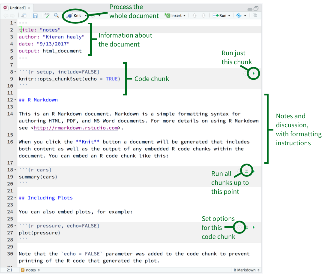
* Each code chunk has several options to interact with
* By clicking the green play button on the top right corner of the chunk, you can run everything in *only* that chunk
* You can also click the downward pointing triangle to run every code chunk above. This is useful for catching up with previous work
* The gear icon will allow you set individual code chunk options
Using rmarkdown reinforces **literate programming**. Writing documentation with executable code in a single document.
Great for reproduciblity!
**Calculating and embedding statistics into your manuscript using R Markdown**
R Markdown language also allows you to embed r code directly into the text of your statistical report. This can save you a LOT of time that you might have spent double and triple checking that you have the most updated values of means, standard deviations, etc. in your written manuscript. See below:
```{r}
The mean speed is `r mean(cars$speed)` (SD= `r round(sd(cars$speed), 2)`).
```
will compile as: "The mean speed is 15.4 (SD= 5.29)."
**R Markdown External Resources:**
For help with markdown language: http://rmarkdown.rstudio.com. You can also find an R Markdown cheatsheet under the help section in RStudio.
**R Markdown Gallery:** https://rmarkdown.rstudio.com/gallery.html
> **Why should we use an R script file instead of a R Markdown file or vice versa?** R scripts are useful for exploratory analysis or for storing repetitive code. R Markdown files are geared towards creating reports or professional documents.
****
## Seeking Help
Besides the Help pane mentioned earlier, we can use the console to ask for a description of a partiuclar function or package.
For example, if we wanted to explore the `mean()` function, we could type `?mean` into the console to get the following:
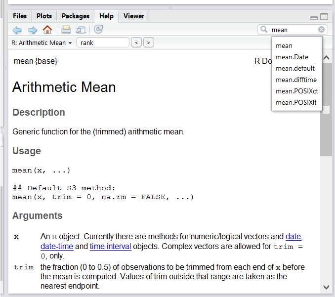
Here we can explore what parameters `mean()` takes and what kind of output we should expect.
## Challenge
Look at the help for `paste`. What is the difference between the `sep` and `collapse` arguments?
* **sep:**
* A character string to separate the terms. Not NA_character_.
* **collapse:**
* An optional character string to separate the results. Not NA_character_.
I agree😊
Yeah... but what does that _mean_??
****
**running code chunks:**
1. use green "play" triangle on the top right of the code chunks.
2. use keyboard commands ``crtl/cmd-enter``
**Note:**
do not hightlight lines and run. you may get an error
**Tip - turn off console output to not display in cosole**
tools/global options/rmarkdown
uncheck "show output inline"
## Data structures
1. Open a new R.text file
coat,weight,likes_string
calico,2.1,1
black,5.0,0
tabby,3.2,1
2. Read in the cats data set
* You must use the function `read.csv()`
* Specify the file location that you would like to read from inside the parentheses
* You must either have the file in your current working directory or specify the path to the file you need to read from
```{r}
cats <- read.csv(file="feline-data.csv")
```
What happens if we just asked for `weight` without specifying the data set?
```{r}
weight
```
matrix vs dataframe = speed when working with data.
## Exploring data frames
**Reading in gapminder dataset**
use read.csv function:
``gapminder <- read.csv("data/gapminder-FiveYearData.csv")``
**note:**
reading in data from the web can be a problem.
every time you run knit, the data will be redownloaded from the link.
looking at structure of the dataset:
``str(gapminder)``
``nrow`` - number of rows
``ncol`` - number of columns
knit code inline in text by using back ticks
e.g. there are `r nrow(gapminder)` observations and `r ncol(gapminder)` in the gapminder dataset.
function to only show variables names:
`colnames(gapminder)` only shows variable names
if you just want to look at top few rows of the data set use the `head` function.
dollar sign notation to access variables vs position e.g. `head(gapminder)`
`gapminder$pop` will print the entire list of population numbers
`head(gapminder$pop)` will only show the first few entries starting at the top.
`head` is based on a Shell command to display only the first several entries in a data file.
`head(gapminder[,3])` access data by position instead of name.
## Challenge question:
Read the output of `str(gapminder)` again; this time, use what you've learned about factors as well as the output of functions like `colnames` and `dim` to explain what everthing that `str` prints out.
* Number of observations
* Type of variable
* How many variables
* First few observations
* `dim` - pulls out the number of observations and how many variables
dim() does in one step what nrow() and ncol() do in two steps
142 countries across 5 continents
**vectorization (or vectorwise operations)**
make a new variable called `logpop` that take the logarithm of the variable `pop` using the function 'log[]'
-first use `cbind` to din gthe columns together
```
gapminder$logpop <- log(gapminder$pop)
```
confirm it's right by looking a the top few rows
```
head(cbind(gapminder$pop, gapminder$logpop))
```
elementwise operations are **different** than summarizing functions lie the mean.
## Challenge 2
Make a new column in the gapminder data frame that conatins population in units of millions of people. Use head or tail of the data fram to make sure it works.
## Functions
functions have aguments.
arguments can be specified positionally or by name.
```
mean(x=gapminder$pop)
```
this is positional
```
mean(gapminder$pop, TRUE)
```
```
mean(gapminder$pop, na.rm=TRUE)
```
same as:
all positional need value for trim
```
mean(gapminder$pop, 0, TRUE)
```
# Day 2 Morning
## Unix Shell
[Download Shell data](http://swcarpentry.github.io/shell-novice/data/data-shell.zip)
references:
[https://explainshell.com/](https://explainshell.com/)
Basic commands:
[http://swcarpentry.github.io/shell-novice/reference/](http://swcarpentry.github.io/shell-novice/reference/)
****
## What is Bash?
* A **command line interface** (CLI) that allows you to quickly type commands and navigate through your file directory.
* Bash is a newer version of the Bourne shell which was originally developed by Stephen Bourne in 1979 at Bell Labs for Unix version 7.
## Why should we use a CLI?
* GUIs (Graphical User Interface) aren't always the quickest way to navigate through files or interact with your computer.
* When working with offsite servers it is common that CLIs will be the only way to use the system.
****
## File Hierarchy

* Files are stored into folders which can be stored in even bigger folders. Instead of clicking like we would in GUI file explorers, Bash will let us type commands to traverse the system.
****
## Basic Commands
* `whoami` prints username of currently logged in user
* `pwd` prints the working directory (i.e. the folder bash is "looking" in)
* `cd` change directory. Use this to move into different folders or move back
* `cd ..` will take you back to the parent directory (where you came from)
* You can also specify the entire path to reduce the amount of times you have to type `cd`
* Ex: `cd /c/Users/my_name/Desktop/SWC_workshop`
* `ls` lists the files and folders in the current directory
* `clear` clears the console, leaving only the command line
* `cp` followed by a filename and a destination will copy the given folder to the location you specify
* `cp notes.txt notes_2.txt` will copy the contents of `notes.txt` and paste it into a newly created `notes_2.txt`
* `mv` will allow to move a file to a specified location
* `mv notes.txt writing/` will move the file into the `writng/` folder
* You will also use `mv` to rename files. Typing `mv notes.txt new_notes.txt` will rename `notes.txt`
* `rm` will delete files that you specify
* **Be careful!** Unix does not have a trash bin so it be very difficult if not impossible to recover files deleted from the command line
* `sort` will sort the contents of a specified file
* The default sorting method is alphabetical. To sort numerically use the flag `-n`
* `cat` will display the contents of a file
* `head` will display the first ten lines of a given file
* Similarly `tail` will display the *last* ten lines
* `man` will prompt you to specify what manual you want
* `man ls` ? retrieves the manual for the ls command, which will tell you what flags/options are available for that command (see <a href= "#bashhelp">Getting Help with Bash</a> below.)
**What does the `.` do?**
* `.` refers to your current location or your *current working directory*
* `..` refers to the parent folder of your current location
* **Be aware** - `.` in front of a file name means the file is *hidden*
**What does the `~` do?**
* `~` refers to your `home` directory. You can use this to retrieve files that stem from home
**What does `-` do?**
* `-` will allow you do move down the file hierarchy. This is dependent on your history of commands, so use it if you need to get back down the tree quickly.
**Autocomplete file names to save time!**
* Type first few letters of the file or folder name and then click `tab`
> Flags are additional parameters you can pass to a command. Use a `-` followed by a key character to utilize them. A command followed with`--help` will detail the various flags you can use.
****
## <a id="bashhelp">Getting Help with Bash</a>
* `man` command will provide a detailed description of the command you would like to know about. For example, `man ls` will generate the manual that describes how `ls` functions as well as the flags that you can utilize.
* To exit the manual in bash, type `q` for "quit."
* As of now, Git Bash for Windows does not recongize the command `man`. For now you can use: https://linux.die.net/man/
* Website: https://explainshell.com/
****
## Exercise #1
Starting from `/Users/amanda/data/`, which of the following commands could Amanda use to navigate to her home directory, which is `/Users/amanda`?
1. `cd .`
2. `cd /`
3. `cd /home/amanda`
4. `cd ../..`
5. `cd ~`
6. `cd home`
7. `cd ~/data/..`
8. `cd`
9. `cd ..`
**Solution**
*5, 7, 8, 9*
****
## Exercise #2
Using the filesystem diagram below, if `pwd` displays `Users/thing`, what will `ls -F ../backup display`?
1. `../backup: No such file or directory`
2. `2012-12-01 2013-01-08 2013-01-27`
3. `2012-12-01/ 2013-01-08/ 2013-01-27/`
4. `original/ pnas_final/ pnas_sub/`

**Solution**
1. No: there is a directory backup in `/Users`
2. No: this is the content of `Users/thing/backup`, but with `..` we asked for one level further up
3. No: see previous explanation
4. Yes: `../backup/` refers to `/Users/backup/`
****
## Creating Directories
* `mkdir` will make a new directory given a name. If we wanted to create a folder called `coursework`, we would type `mkdir coursework`
* **Keep file names short**
* Bash requires a lot of typing so by making short names with simple characters will make your life easier!
* Its good practice to eliminate spaces and stick to either CamelCase or snake_case
> To remove a directory you cannot simply use `rm` as you can with files. You must first delete all files contained in the directory before Bash will allow you to remove it. Use `rmdir` on an empty directory to delete it.
****
## Editing Files
In this workshop we'll be using the text editor `nano`. There are other popular text editors but `nano` is simple to use and readily available. To launch from the command line type `nano` followed by the file you wish to create or edit.
**Example**
```{bash}
nano new_file.txt
```

> The `^` symbolizes `CTRL`. Therefore to exit the text editor type `CTRL` + `X`
**Tips**
* `CTRL` + `O` will allow to save your file
* `CTRL` + `X` to exit
****
## Exercise #3
Suppose that you created a `.txt` file in your current directory to contain a list of the statistical tests you will need to do to analyze your data, and named it: `statstics.txt`.
After creating and saving this file you realize you misspelled the filename! You want to correct the mistake, which of the following commands could you use to do so?
1. `cp statstics.txt statistics.txt`
2. `mv statstics.txt statistics.txt`
3. `mv statstics.txt .`
4. `cp statstics.txt .`
**Solution**
1. No. While this would create a file with the correct name, the incorrectly named file still exists in the directory and would need to be deleted.
2. Yes, this would work to rename the file.
3. No, the period(.) indicates where to move the file, but does not provide a new file name; identical file names cannot be created.
4. No, the period(.) indicates where to copy the file, but does not provide a new file name; identical file names cannot be created.
****
## Wildcards, Pipes, and Filters
### Wildcards
Wildcards are characters that have special functions.
* `*` matches *zero or more* characters. If we used the command `ls *.txt`, all of the files that have zero or more characters preceding `.txt` will be listed. This has the effect of only listing `.txt` files
* `>` will redirect the output of a command into a file
* Let's breakdown the following command:`wc *.txt > lengths.txt`. `wc` will generate the number of lines, words, and characters for a given file. Since we used `*.txt` this command will be applied to each `.txt` file. This entire output will be fed into a new file called `lengths.txt`
* This is handy for saving output from a command or simply for easier viewing. Your console will get crowded from various commands so by directing output to files you can stay organized
### Pipes
Bash provides built in features that allow you to link commands together. By taking the output of one command and using it as the input for another we can do some cool stuff!
* `|` takes the output of the command on the left and uses it as the input of the command on the right
* **Ex:** To get the third line of a file you can use pipes: `head -3 sortedLengths.txt | tail -1`

****
## Scripts
Sometimes it can be useful to have a series of commands saved as a script, which you can call upon later. When called a script will execute the commands saved inside.
* Create a script file in nano by using the extension `.sh`
* Ex: `$ nano sample.sh` will open nano, where you can create your script
* Execute a script by using the command `bash`
* **Ex:** `bash sample_script.sh`
* Use `$` to reference filenames that you can pass to your script
* Inside a shell script, $1 means “the first filename (or other argument) on the command line”
* Typing `#` allows you to make a comment. Comments will not be interpreted by the machine so its useful for making notes or even rendering a block of code inert without deleting it.
```{bash}
$ bash middle.sh octane.pdb
```
Now, if we open up `middle.sh`, we can reference octane.pdb without directly using its name. This means we can now pass any file!
```{bash}
head -n 15 "$1" | tail -n 5 # $1 refers to octane.pdb
```
> Comments allow you to come back at a later time and view notes you made about your code. Remember that you may not be the only person who will read this, so by documen your code with comments so it is easy to understand.
****
# Day 2 Afternoon
## Data Visualization
The three standard choices
* **Base Graphics**- Very basic graphs used and seen only by the statistion as a way to understand your data
* `plot()`
* `hist()`
* **Lattice** - provides better default graphs and the ability to easily display multivariate relationships
* Learn more: https://www.statmethods.net/advgraphs/trellis.html
* **ggplot**- Used most frequently to showcase your data/finding in an aestheticly pleasing way.
* Learn more: https://www.statmethods.net/advgraphs/ggplot2.html
****
## Creating Plots with ggplot
> When reading data, always make sure that you are referencing the correct file path. A good practice is to simply type the full path to your data when using `read.csv()`.
**Try this** after loading data in gapminder
```{r}
ggplot(data = gapminder, aes(x = gdpPercap, y = lifeExp)) + geom_point()
```
What happens?
## Common Errors
### Forgetting to load in library
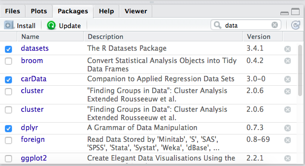
* Load in library in the code chunk!
**Example:**
```{r}
library(ggplot2)
```
> While you can load the library from the console, it is a good habit to include this line of code directly in your scripts or R Markdown file. This will ensure your code will run the way you expect it to.
### Cannot open connection
If you get an error that claims a connection cannot be made, most likely it is because it can't find your file. Correct the path to the file your are reading your data from and the error should be resolved.
### Look out for `+` placement in ggplot
The `+` operator goes between ggplot layers. It's a common mistake to have a trailing `+`.
****
**Structure**
A key strength of ggplot2 is its ability to layer graphs. Each new layer is denoted by a `+`. Notice above `+ geom_point()`. This layer specifies we want to graph *points*.
* `data` - the name of your dataframe or dataset that you want to use
* `aes()` - aesthetics. This is wher you will specify your x-axis and y-axis
* `+ geom_point()` - A specfic layer added on to ggplot to create a scatter plot.
* **Note** that there are a lot of different layers to add on to ggplot to make a plethera of different graphs.
****
## Challenge 1
Modify the example so that the figure visualise how life expectancy has changed over time:
```{r}
ggplot(data = gapminder, aes(x = gdpPercap, y = lifeExp)) + geom_point()
```
>Hint: the gapminder dataset has a column called “year”, which should appear on the x-axis.
**Solution**
```{r}
ggplot(data = gapminder, aes(x = year, y = lifeExp)) + geom_point()
```

****
## Challenge 2
Using a scatterplot probably isn’t the best for visualizing change over time. Instead, let’s tell ggplot to visualize the data as a line plot:
```{r}
ggplot(data = gapminder, aes(x=year, y=lifeExp, by=country, color=continent)) +
geom_line()
```
> The **by** *aesthetic* tells ggplot group by something and `geom_line` draws a line through that something.
**solution**
```{r}
ggplot(data = gapminder, aes(x = year, y = lifeExp, color=continent)) +
geom_point()
```

****
## Layers
```
ggplot(data = gapminder, aes(x = gdpPercap, y = lifeExp, color=continent)) +
geom_point()
```
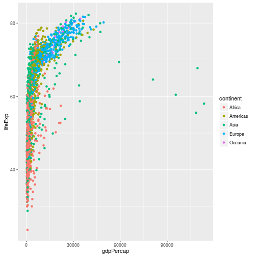
By performing a log transformation, we can scale the graph to make interpretation easier
```
ggplot(data = gapminder, aes(x = gdpPercap, y = lifeExp)) +
geom_point(alpha = 0.5) + scale_x_log10()
```
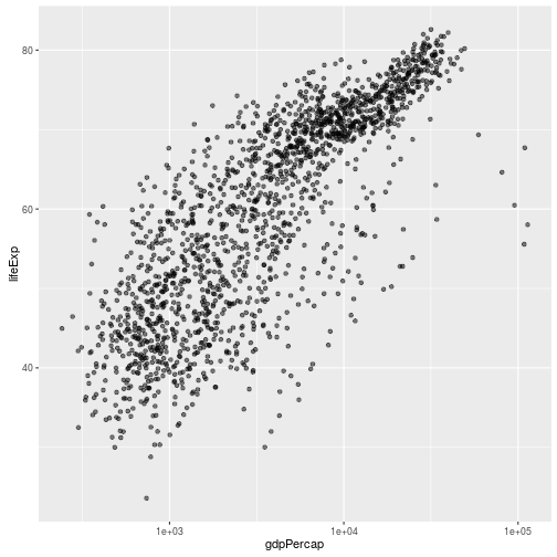
We can also add another layer to fit a relationship using `geom_smooth()`.
```
ggplot(data = gapminder, aes(x = gdpPercap, y = lifeExp)) +
geom_point() + scale_x_log10() + geom_smooth(method="lm")
```
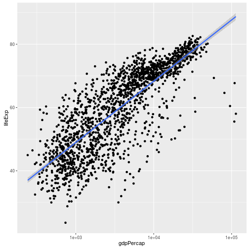
> Here we are specifying `method="lm"` indicating we want to represent a linear relationship.
## Challenge 4a
Modify the color and size of the points on the point layer in the previous example.
>Hint: do not use the `aes` function.
**Solution**
```ggplot(data = gapminder, aes(x = gdpPercap, y = lifeExp)) +
geom_point(size=3, color="orange") + scale_x_log10() +
geom_smooth(method="lm", size=1.5)
```
## Challenge 4b
Modify your solution to Challenge 4a so that the points are now a different shape and are colored by continent with new trendlines. Hint: The color argument can be used inside the aesthetic.
**Solution**
```ggplot(data = gapminder, aes(x = gdpPercap, y = lifeExp, color = continent)) +
geom_point(size=3, pch=17) + scale_x_log10() +
geom_smooth(method="lm", size=1.5)
```
****
## Paneling
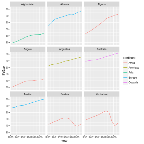
We can feature subsets of our data using panels
```{r}
starts.with <- substr(gapminder$country, start = 1, stop = 1)
az.countries <- gapminder[starts.with %in% c("A", "Z"), ]
ggplot(data = az.countries, aes(x = year, y = lifeExp, color=continent)) +
geom_line() + facet_wrap( ~ country)
```
* `facet_wrap()`- subsets graph based on a varable in your dataset
## Modifying Text
To clean this figure up for a publication we need to change some of the text elements. The x-axis is too cluttered, and the y axis should read “Life expectancy”, rather than the column name in the data frame.
We can do this by adding a couple of different layers. The `theme()` layer controls the axis text, and overall text size, and there are special layers for changing the axis labels. To change the legend title, we need to use the `scales` layer.
```{r}
ggplot(data = az.countries, aes(x = year, y = lifeExp, color=continent)) +
geom_line() + facet_wrap( ~ country) +
xlab("Year") + ylab("Life expectancy") + ggtitle("Figure 1") +
scale_colour_discrete(name="Continent") +
theme(axis.text.x=element_blank(), axis.ticks.x=element_blank())
```
* `xlab()`- Changes the x-axis lable
* `ylab()`- Changes the y-axis lable
* `ggtitle()`- Adds a title to your graph
* `scale_colour_discrete()`- Allows you to change the name of your table
****
## Help with ggplot
* Cookbook for R
* http://www.cookbook-r.com/Graphs/
* R Studio has add-ins
* https://github.com/calligross/ggthemeassist
* Intro to R "full data viz tutorial"
* https://norcalbiostat.github.io/MATH130/full_data_viz_tutorial.html
****
## Dataframe Manipulation with `dplyr`
### Base R manipulation
```{r}
mean(gapminder[gapminder$continent == "Africa", "gdpPercap"])
```
Here we can select the continent *Africa* by using the `==` operator. However, when having to repeat this command for multiple contintents it can become repetitive. Luckily there's a better way
The five most common funtions in `dplyr`
1. `select()`
2. `filter()`
3. `group_by()`
4. `summarize()`
5. `mutate()`
> Don't forget to load `dplyr`!
****
### Using `select()`
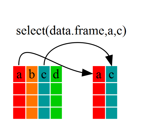
Select grabs **columns**
```{r}
year_country_gdp <- select(gapminder,year,country,gdpPercap)
```
or with a pipe
```{r}
year_country_gdp <- gapminder %>% select(year,country,gdpPercap)
```
Used to extract certain varables(columns) from a dataset makeing a new, usually smaller, dataset.
****
### Using `filter()`
Filter selects **rows**
```{r}
year_country_gdp_euro <- gapminder %>%
filter(continent=="Europe") %>%
select(year,country,gdpPercap)
```
> Notice how we use `%>%` to feed the output from `filter()` to `select()`. This is similar in function to the pipe operator from Bash. The shortcut for `%>%` is `CTRL+SHIFT+M`
### Challenge
Write a single command (which can span multiple lines and includes pipes) that will produce a dataframe that has the African values for `lifeExp`, `country` and `year`, but not for other Continents. How many rows does your dataframe have and why?
Answers:
```{r}
year_country_gdp_afri <- gapminder %>%
filter(continent=="Africa") %>%
select(lifeExp, country, year)
```
```{r}
year_country_gdp_afri <- gapminder %>%
filter(continent=="Africa") %>%
select(lifeExp, country, year)
```
```{r}
year_country_gdp_africa <- gapminder %>%
filter(continent=="Africa") %>%
select(year, country, lifeExp)
```
You can use the `nrow` command to find the number of rows, or you could use the `dim` command that will output the number of rows and columns.
* 624 rows, 3 columns
****
### Using `group_by()` and `summarize()`

```{r}
gdp_bycontinent <- gapminder %>%
group_by(continent) %>%
summarize(mean_gdpPercap = mean(gdpPercap))
```

### Challenge
Calculate the average life expectancy per country. Which had the longest life expectancy and which had the shortest life expectancy?
**Solution**
```{r}
lifeExp_bycountry <- gapminder %>%
group_by(country) %>%
summarize(mean_lifeExp=mean(lifeExp))
```
```{r echo=FALSE}
life_expentacy_bycountry <- gapminder %>%
group_by(country) %>%
summarise(mean_lifeExp = mean(lifeExp))
head(life_expentacy_bycountry)
```
```
life_bycountry <- gapminder %>% group_by(country) %>% summarize(mean_life_exp = mean(lifeExp)) %>% arrange(mean_life_exp)
```
* You can group by multiple variables
**Example:**
```{r}
gdp_bycontinents_byyear <- gapminder %>%
group_by(continent,year) %>%
summarize(mean_gdpPercap=mean(gdpPercap))
```
* You can also define more than one variable in `summarize()`
**Example:**
calculate the gdp per capita by continents and by year
```{r}
gdp_pop_bycontinents_byyear <- gapminder %>%
group_by(continent,year) %>%
summarize(mean_gdpPercap=mean(gdpPercap),
sd_gdpPercap=sd(gdpPercap),
mean_pop=mean(pop),
sd_pop=sd(pop))
```
****
## Using `mutate()`
We can also create new variables prior to (or even after) summarizing information using `mutate()`.
```{r}
gdp_pop_bycontinents_byyear <- gapminder %>%
mutate(gdp_billion=gdpPercap*pop/10^9) %>%
group_by(continent,year) %>%
summarize(mean_gdpPercap=mean(gdpPercap),
sd_gdpPercap=sd(gdpPercap),
mean_pop=mean(pop),
sd_pop=sd(pop),
mean_gdp_billion=mean(gdp_billion),
sd_gdp_billion=sd(gdp_billion))
```
## Challenge
Take the data set you just created `gdp_pop_bycontinents_byyear`, and create a line plot (scatterplot where the points are connected with lines) to look at the how the average population (`mean_pop`) change across years, for each continent. Use either `color` or `shape` on the continents to get a legend to appear.
**Solution**
```
ggplot(data = gdp_pop_bycontinents_byyear, aes(x = year, y = mean_pop, by=continent)) +
geom_line(aes(color=continent)) +
geom_point()
```
## Advanced Challenge - BEWARE!
Using pipes, filter `gdp_pop_bycontinents_byyear` so to only include records for continents with average population lower than 50 million. (`mean_pop < 5*10^7`). Instead of saving this as a new data set and then calling `ggplot()` on that new data set, pipe the `ggplot()` function directly after the `filter()` statement. Be sure to remove the first argument to ggplot (the data set name), since that's the purpose of the piping!
**Solution**
```
gdp_pop_bycontinents_byyear %>% filter(mean_pop <5*10^7) %>%
ggplot(aes(x=year, y=mean_pop, color=continent)) + geom_line()
```
****
# Day 3 - Optional
## Version Control
### Github usernames
* Naomi: nstamper :smile_cat:
* Stephanie: sbianco4022
* Kathleen🤩: kjohnson156
* Zach: zherrnstadt
* Grant: gesparza3
* Eisley: eisleyadore
* Jerry: mathistite
* Shelley: srhart73
* Reid: u2ng
****
### What is version control?
Version control allows us to make sequential changes to projects. Git will track our changes making it easy to jump back to older versions of a project.
#### References
* http://happygitwithr.com/hello-git.html
#### Vocabulary
* **local**: something on your computer
* **remote**: something living online, in a place like GitHub
* **git**: version control software
* **GitHub**: online storage repository for version control folders
* `git add`: Add files and changes to a "staging area"
* `git commit`: Record your changes to a file (or set of files). Each commit records an ID number that allows changes to be tracked
* `git push`: Send your committed changes to a remote repository, such as a repository hosted on GitHub.
* `git pull`: copy new changes from a remote repository down to your local machine.
* **repository**: a folder that is being tracked under version control
* **clone**: make a copy of a remote repository onto your local machine.
* **fork**: make an entire copy of someone elses git repo, into your account. This repo is then linked back "upstream" to the original users account.
* This is how collaboration is done. One person has the master version of a repo (for a website, software program etc), other collaborators _fork_ this repo to have their own copy. They work on the project, and then submit **pull requests** back to the original owner to ask to have their changes incorporated.
#### Benefits
* Changes are tracked
* New *branches* of a project can be created
* All of your files will be backed up
* "Easily" merge changes across a project
****
### Creating your Git environment
#### 1. Link your account
In the shell (Appendix A) type the following
* `git config --global user.name "your name here"`
* `git config --global user.email "your github email"`
confirm your setup right
* `git config --global --list`
Example:
git config --global user.name "norcalbiostat"
git config --global user.email "rdonatello@csuchico.edu"
git config --global --list
#### 2. Define line ending
For mac users:
`git config --global core.autocrlf input`
For windows users:
`git config --global core.autocrlf true`
#### 3. Configure git editor
`git config --global core.editor "nano -w"`
****
## Working with Git
We have only covered the git basics `setup, add, commit, push, pull`.
[Full Git lesson notes here](http://swcarpentry.github.io/git-novice/)
* `git init` into your current working directory to initialize an empty **repository**
> A **repository** is where your projects will live. Our repositories will be hosted on Github. Initialization tells Git that we're ready to start a new project.
* `git status` will tell you exactly where you are in the version control process. This is an extremely useful command and one that you will use often
* Files marked in red indicate the files are *not* being tracked
* Files marked in green *are* being tracked
* `git add` will tell Git to you want this file to be tracked
* `git commit -m "Your commit message"` will keep a record of your changes. You must enter a commit message to describe the changes you made
* `git log` will show you your recent changes that have been logged
* `git diff` will allow you to see the changes made to your file before making a commit
### Github
In order to connect our locally stored projets to Github's servers, we need to navigate to Github.com
After logging into your account, create a new repository by clicking the `+` button on the top right of the page.
> Use the same name for your online repository and your local copy. This will save you many headaches
Once your repository is sucessfully added to your account, go back to the terminal type the following:
```
git remote add origin [url of your Github repository]
```
## Website building using Git through R Studio
This is for building basic websites using Rmarkdown.
1. Make new repo in github. Initalize with a readme
2. Open R Studio
3. Create a new project
- version control
- git
4. Go back to Github. Click the green clone or download button at the top of your repo to copy the URL.
- Paste into R Studio
- open in new session optional
5. Start a new R text file.
- Save this file as as `_site.yml`
- copy the following code into this file.
> note: indentation matters when creating this .yml file. You must keep tab indent formatting as shown below.
```
name: "Robin Dontello"
output_dir: "."
navbar:
title: "SWC workshop webpage"
left:
- text: "Schedule"
icon: fa-database
href: http://example.com
right:
- text: "Syllabus"
icon: fa-info-circle
href: syllabus.html
output:
html_document:
theme: yeti
highlight: tango
lib_dir: site_libs
self_contained: no
```
6. Start a new R Markdown file.
- Give it a title
- delete template text **Keep the header material**
- Write "hello world"
- Save as `index.Rmd`
7. Restart R Studio
This will allow R studio to recognize that the folder now has "instructions" contained in the `_site.yml` file that tell it what to do.
- Click the `build` tab in the upper right.
- Click build website.
You can see the preview in the viewer window, but let's make it live!
8. Commit your changes
a. Using the Git tab gui interface.
- click the `diff` icon
- `ctrl+A` to select all.
- check `stage` button
- commit message "initial site build"
- commit + push
b. Commit your changes using shell commands.
- Click on the `Terminal` tab next to your console.
- `git add -A`
- `git commit -m "initial commit"`
- `git push`
9. In Github go to your site repo.
- Click on settings icon at the top
- Scroll down to the Github pages section, near the bottom.
- select source `master branch`, then click save.
- Scroll back down to Github pages.
- Click on URL to your live site.
Github will auto generate a site link in the Github Pages section in this format:
`http://[yourusername].github.io/[sitereponame]`
It's recommended to copy this URL and add it to your repo description.
---
### Considerations for websites
* Everything in a public repo is PUBLIC. Don't put sensitive info in there.
* Everything in the same folder as `index.rmd` will be compiled/knit when you click `build website`
* Files in subfolders will not.
* use scripts to help manage which files need to be built each time.
* Start small, copy something that works and build off of it.
* Think long about design and file structure BEFORE you start building too much.
* Links to other files (like word docs etc) are typically hard coded in like this: `[link title](URL or file path)`. These will break if the file is moved. Capitalization matters here too.
* Don't get too hung up on little things (like color themes).
---
## Follow people in Github
Under the person's profile picture, there is a **Follow** button. You will see their updates in a feed like system when you log into github.
A small selection of instructors who host class materials on GitHub
* Mine Cetinkaya at Duke https://github.com/mine-cetinkaya-rundel
* http://www2.stat.duke.edu/courses/Spring18/Sta199/
* Jenny Bryan at University of British Columbia https://github.com/jennybc
* http://stat545.com/
* Robin Donatello at CSUC https://github.com/norcalbiostat
* http://www.norcalbiostat.com/#teaching
* Carl Boettiger https://github.com/cboettig
* https://espm-157.carlboettiger.info/
## Etiquitte on sharing materials
If it's on github in a public repo, it means you are welcome to take a copy of their work.
Check for any licenses they may have, some may restrict copying to disallow any re-use of their work for profit. More information about the Creative Common licences allow see their website https://creativecommons.org/licenses/
To make a copy of someone elses' repo, click on the **Fork** button. This will copy ALL the contents of their repository into your github account. You can then work on your own copy.
If you decide to publish a repo based on someone elses work, it is proper etiquitte to acknowledge their contribution in the `readme.md` file.
---
# Learning resources
General
* Software Carpentry https://software-carpentry.org/
* Data Carpentry https://datacarpentry.org/
* Data Science Initative at Chico State workshops and seminars http://datascience.csuchico.edu/
* Data Camp: Learn R, Python, SQL, other Data Science languages https://www.datacamp.com/home
Version control
* Using git, github and R http://happygitwithr.com/
* Atlassian Git tutorials and training https://www.atlassian.com/git/tutorials
R/R Markdown
* R Studio tutorials: https://www.rstudio.com/online-learning/
* The Definitive guide to RMarkdown https://bookdown.org/yihui/rmarkdown/
* Creating Books using Rmarkdown https://bookdown.org/yihui/blogdown/

