2019q1 Homework7 (skiplist)
===
contributed by < `Laurora` >

---

### 測驗 `1`

給定一個 circular linked list 實作如下: (檔案 `list.h`)

#ifndef INTERNAL_LIST_H
#define INTERNAL_LIST_H

/* circular doubly-linked list */
typedef struct __list_t {
    struct __list_t *prev, *next;
} list_t;

/*
 * Initialize a list to empty. Because these are circular lists, an "empty"
 * list is an entry where both links point to itself. This makes insertion
 * and removal simpler because they do not need any branches.
 */
static inline void list_init(list_t *list) {
    list->prev = list;
    list->next = list;
}

/*
 * Append the provided entry to the end of the list. This assumes the entry
 * is not in a list already because it overwrites the linked list pointers.
 */
static inline void list_push(list_t *list, list_t *entry) {
    list_t *prev = list->prev;
    entry->prev = prev;
    entry->next = list;
    prev->next = entry;
    list->prev = entry;
}

/*
 * Remove the provided entry from whichever list it is currently in. This
 * assumes that the entry is in a list. You do not need to provide the list
 * because the lists are circular, so the list's pointers will automatically
 * be updated if the first or last entries are removed.
 */
static inline void list_remove(list_t *entry) {
    list_t *prev = entry->prev;
    list_t *next = entry->next;
    prev->next = next;
    next->prev = prev;
}

/*
 * Remove and return the first entry in the list or NULL if the list is empty.
 */
static inline list_t *list_pop(list_t *list) {
    list_t *foo = list->prev;
    if (foo == list)
        return NULL;
    LL1
}
#endif

請參照上方程式註解，補完對應程式碼。

要求補完的程式碼是 `list_pop` ，由於選項是要利用 `list_remove` 實作 `list_pop` ，因此我們先看 `list_remove` 是怎麼運作的

/*
 * Remove the provided entry from whichever list it is currently in. This
 * assumes that the entry is in a list. You do not need to provide the list
 * because the lists are circular, so the list's pointers will automatically
 * be updated if the first or last entries are removed.
 */
static inline void list_remove(list_t *entry) {
    list_t *prev = entry->prev;
    list_t *next = entry->next;
    prev->next = next;
    next->prev = prev;
}

* 在 list 的 `entry->prev` 新增 `*prev` ，如下圖

list_t *prev = entry->prev;


* 在 list 的 `entry->next` 新增 `*next`

list_t *next = entry->next;


* 將 `prev->next` 指向 `next`

prev->next = next;


* 將 `next->prev` 指向 `prev`

prev->next = next;


這樣就完成一次 remove entry ，不過這邊似乎沒有將 entry 所指向的 `prev` 和 `next` 指向 `NULL`，實作的時候需要注意這點。

再來看 `list_pop`

/*
 * Remove and return the first entry in the list or NULL if the list is empty.
 */
static inline list_t *list_pop(list_t *list) {
    list_t *foo = list->prev;
    if (foo == list)
        return NULL;
    LL1
}

註解的要求是要將 list 的 first entry 移除並回傳。
`list_t *foo = list->prev;` 這裡的 `*foo` 就是 list 的 first entry，一次 `list_remove(foo)` 後就可以移除，之後 `return foo;` 即可。
因此答案選 (e) `list_remove(foo); return foo;`

---

### 延伸問題

#### 1.研讀 2019q3 Week11 的 cache-oblivious data structures 參考資料，記錄所見所聞
[**Maximize Cache Performance with this One Weird Trick: An Introduction to Cache-Oblivious Data Structures**](https://rcoh.me/posts/cache-oblivious-datastructures/)
一般在學習演算法時，Big-O 的概念大多側重於整個程式運算的次數，是因為有一個大前提：假設從記憶體存取的時間成本與讀取的位元組 (byte) 成正比。但是實際上計算機的存取單位是資料段 (block) ，為了更貼近計算機存取的實際情況，於是就有了這個考慮硬體存取成本的模型。
* 假設在記憶體有 2 個分層: 小快速層(通常為 cache)、大慢速層(通常為 disk)
* 慢速層記憶體無限大；快速層大小為 $M$ ，且無限快
* 記憶體只能以大小為 $B$ 的資料段從慢速層移動到快速層
* $M$ 和 $B$ 可為任意值
* 只分析最慢層到次慢層的傳遞，其他視為更快的傳遞，不影響結果

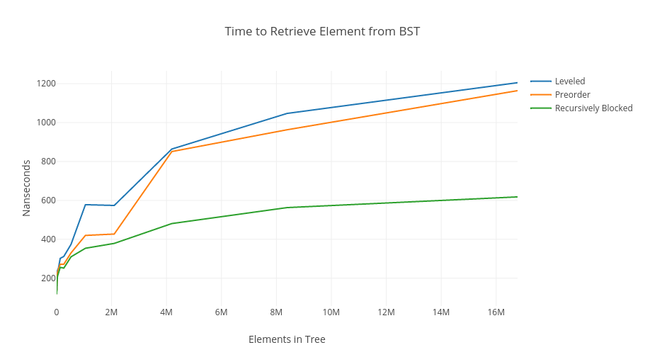
上圖可以發現，不同演算法在樹的大小越大而分歧越大。當樹很小，三者還看不出分歧時，表示這棵樹可以很完美的存在一個資料段中；圖中線段還有比平坦的部分在特定的 cache 大小時會發生；而樹越來越大， Cache-Oblivious 演算法的優勢就越明顯。

**藍色線段: Leveled (BFS)**
* 樹中的樹字指的是元素在字組中的位置，橙色框為記憶體中的分組
* 以記憶體的角度是一個很糟糕的演算法，從根部到葉走訪，一旦一列所含元素太多，會造成每一列都會在不同的資料段中，而每一個資料段僅讀取一個元素，最後會需要讀取 $\log_2N$ 個資料段。

**橙色線段: Preorder (DFS)**
* 最佳情況：沿最左邊走訪(橘色圈部分)比 BFS 好，僅需讀取 1 個資料段
* 最差情況：沿最右邊走訪仍需讀取 $\log_2N$ 個資料段。

**綠色線段: Recursive Block Approach**
* 綠色框為 block，橙色框為 superblock
* 所有的 block 之間==連續==，所有的 superblock 之間也==連續==
* 當讀取的 block 越大，相較之前演算法，讀取的階層會少的越多
* 例：若讀取一個大小為 $B$ 的 block，原來預期會讀取 $\log_2B$ 層才能走訪根到葉，而整個樹有 $\log_2N$ 層，透過 Recursive Block Approach 只需要存取 $\log_BN$ 個 block。
* $\frac{\log_2N}{\log_2B}=\log_BN$

[**Memory Hierarchy Models**
](https://www.youtube.com/watch?v=V3omVLzI0WE)
**extended-memory model (I/O model, Disk Access Model, cache-aware model)**
1. 記憶體階層的記憶體大小 (size) 與傳遞時間 (latency) 通常隨深度(階層距離 cpu 越遠)呈指數成長
2. 計算 latency: 最後一層與倒數第二層之間的 memory transfer 即可，在這裡是 disk 和 cache 之間的傳遞 (假設存取 cache 為無限快)
3. $\frac{ number\ of\ cell\ probes}{B}\leqq$ number of memory transfer $\leqq$ RAM running time

> RAM running time: 在 RAM 中每一次運算都當作一次 memory transfer
> number of cell probes: 在一次運算中需要讀取幾個字組

4. 計算 memory transfer
- [Scanning](https://youtu.be/V3omVLzI0WE?t=500): $O(\lceil\frac{N}{B}\rceil)$
- [Search trees](https://youtu.be/V3omVLzI0WE?t=553) (B-tree): $O(\log_{B+1}N)$、$\Omega(\log_{B+1}N)$
- [Sorting](https://youtu.be/V3omVLzI0WE?t=920): $O(\frac{N}{B}\log_{\frac{M}{B}}\frac{N}{B})$
> 一般 sorting 的最佳解通常是$O(Nlog_2N)$ 在這個模型可以看到明顯的進步
- [Permuting](https://youtu.be/V3omVLzI0WE?t=1041):$O(min\{N,\frac{N}{B}\log_{\frac{N}{B}}\frac{N}{B}\})$
- [Buffer tree](https://youtu.be/V3omVLzI0WE?t=1174): $O(\frac{1}{B}\log_{\frac{M}{B}}\frac{N}{B})$、尋找最小值: $O(\phi)$
> 平攤 memory transfer，用於 delayed queries 和 batch update，此時尋找最小值: $O(\phi)$

**cache-oblivious model**
較新的 Memory Hierarchy Model ，與 extended-memory model 最大的區別是，這個模型的 $M$(cache size) 和 $B$(block size) 未知，因此不能手動計算要讀、寫的 block ，cache 滿的時候也不能決定哪一個 block 要優先被踢出去

1. 演算法
- 與 RAM 演算法相似
- cache 替換可利用 LRU(least resent used)、FIFO(first-in-first-out)等算法可接近最佳解
- 必須適用於各種大小的 $B$、$M$，也就是在每一個記憶體階層間的 memory transfer 都要找的到最佳解

2. 計算 memory transfer
* [Scanning](https://youtu.be/V3omVLzI0WE?t=1849): $O(\lceil\frac{N}{B}\rceil)$
- [Search trees](https://youtu.be/V3omVLzI0WE?t=1867) (B-tree): $O(\log_{B+1}N)$、$\Omega(\log_{B+1}N)$
- [Sorting](https://youtu.be/V3omVLzI0WE?t=1906): $O(\frac{N}{B}\log_{\frac{M}{B}}\frac{N}{B})$
- [Permuting](https://youtu.be/V3omVLzI0WE?t=1041): 找不到最小值。因為無法定義 B 和 M 的關係。
- [Priority Queue](https://youtu.be/V3omVLzI0WE?t=2067): $O(\frac{1}{B}\log_{\frac{M}{B}}\frac{N}{B})$
> tall cache assumption: cache 存取了 M 個物件，其中 $M=\Omega(B^{1+\epsilon})$
3. cache-oblibious static search trees
* 應用平衡二元搜尋樹
* [van Emde Boas 排序](https://youtu.be/V3omVLzI0WE?t=2388)
* 將樹從正中間的階層切一半
* 用遞迴的方式將$\sqrt N$ 的三角形分離出來 (Divide)
* 再將每個三角形連接起來 (Conquer)

* 分析：在知道 B 的情況

* 遞迴條件設定為三角形尺寸 $\lt B$ 就停止
* 切割完後可以保證存取每個三角形最多只需要 $2$ 次 memeory transfer
* 小三角形的高度為 $\theta(\lg B)\in (\frac{1}{2}\lg B, \lg B)$
* 從 root 到 leaf 最多需要經過 $\frac{\lg N}{\frac{1}{2}\lg B}$ 個小三角形
* 所以memory transfer 次數 $\leq 4\log_{B+1}N$

[**Skip list**](https://en.wikipedia.org/wiki/Skip_list)
一般的 linked list 搜尋時必須從第一個開始，按照順序一個一個搜尋，因此不論是插入、刪除、搜尋的時間複雜度皆為 $O(\log N)$，而 skip list 可以讓 n 個元素的平均時間複雜度收斂到 $O(\log N)$

**建立 skip list**
1. 最底層 (level 1) 是包含所有元素的 linked list
2. 保留第一個和最後一個元素，從其他元素中隨機選出一些元素形成新的一層 linked list
3. 為剛選出的每個元素新增指標，指向下一層和自己相等的元素
4. 重複 2、3 直到不再能選擇出除了第一個和最後一個元素以外的元素

**特徵**
* 第一層包含所有的元素
* 每一層都是一個有序的 linked list
* skip list 是隨機生成，所以即使元素完全相同的 linked list ，最終的生成的 skip list 有可能不一樣
* 如果元素 x 出現在第 i 層，則所有比 i 小的層都包含 x

**在 skip list 插入元素**

---

#### 2.依據之前給定的 Linux 核心 linked list 實作，開發 cache-oblivious 的版本，並證實其效益;

---

#### 3.實作 Skip list，並且比照之前的 unit test 提供對應的測試、效能分析，還有改善機制