2016q3 Homework 1 (compute-pi)

contributed by <carolc0708>

作業說明A03: compute-pi

學習目標

• [ ]學習透過離散微積分求圓周率
  • Leibniz formula for π
  • 積分計算圓周率π
  • Function
• [ ]著手透過 SIMD 指令作效能最佳化

程式執行結果

學習使用 gnuplot 製圖

在 runtime.gp 中編輯繪圖語法:

reset
set ylabel 'Time(sec)'
set xlabel 'N'
set style fill solid
set title 'wall clock time - using clock_gettime()'
set term png enhanced font 'Verdana,10'
set output 'runtime.png'
set logscale x 10
set datafile separator ","

plot [64:35000][0:] 'result_clock_gettime.csv' using 1:2 smooth csplines lw 2 title 'baseline', \
'' using 1:3 smooth csplines lw 2 title 'omp_2', \
'' using 1:4 smooth csplines lw 2 title 'omp_4', \
'' using 1:5 smooth csplines lw 2 title 'avx', \
'' using 1:6 smooth csplines lw 2 title 'avxunroll', \

在 Makefile 中定義製圖的 rule

plot: gencsv
        gnuplot runtime.gp

執行 $ make plot 後會發現檔案多出一個 runtime.png， 再使用 $ eog runtime.png 即可看到圖像

不同的時間量測方式

• 參考 作業說明 當中的解說，首先須了解 Wall-clock time 和 CPU time 的差別

  • Wall-clock time: 掛鐘時間，真實世界所經過的時間。可能會和 NTP 伺服器、時區、日光節約時間同步或使用者自己調整。
  • CPU time: 程序在 CPU 上面運行消耗 (佔用) 的時間
    • real time : 也就是 Wall-clock time，當然若有其他程式同時在執行，必定會影響到。
    • user time : 表示程式在 user mode 佔用所有的 CPU time 總和。
    • sys time : 表示程式在 kernel mode 佔用所有的 CPU time 總和 ( 直接或間接的系統呼叫 )。
  • 在單一處理器的情況下，可以使用 real - (user + sys) 來計算 Wall-clock time 與 CPU time 的差異。可以理解「所有」可以延遲程式的因子的總和。在 SMP 底下可以近似成 (real * 處理器數目) - (user + sys)。

• clock()

  • the sum of user and system time

• clock_gettime()
  參考 Linux man page，該函式可根據想要取得的 clock 值去做定義，有以下幾種:

  • CLOCK_REALTIME: System-wide realtime clock. Setting this clock requires appropriate privileges.
  • CLOCK_MONOTONIC: Clock that cannot be set and represents monotonic time since some unspecified starting point.
  • CLOCK_PROCESS_CPUTIME_ID: High-resolution per-process timer from the CPU.
  • CLOCK_THREAD_CPUTIME_ID: Thread-specific CPU-time clock.

  在 benchmark_clock_gettime.c 中， clock_gettime(CLOCK_ID, &end) ，其中 CLOCK_ID define 為 CLOCK_MONOTONIC_RAW

  • 資料 中提到，CLOCK_MONOTONIC 和 CLOCK_MONOTONIC_RAW 的不同:
    • CLOCK_MONOTONIC never experiences discontinuities due to NTP time adjustments, but it does change in frequency as NTP learns what error exists between the local oscillator and the upstream servers.
    • CLOCK_MONOTONIC_RAW is simply the local oscillator, not disciplined by NTP.

以不同方式計算圓周率

baseline 版本

• pi 的公式:
  
• 黎曼積分原理:
  
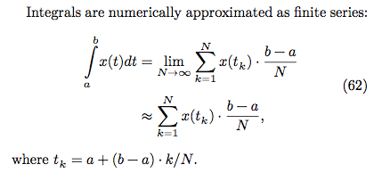
  N 越大代表切得越細，數值越精確
• 程式碼:

double compute_pi_baseline(size_t N)
{
    double pi = 0.0;
    double dt = 1.0 / N;                // dt = (b-a)/N, b = 1, a = 0
    for (size_t i = 0; i < N; i++) {
        double x = (double) i / N;      // x = ti = a+(b-a)*i/N = i/N
        pi += dt / (1.0 + x * x);       // integrate 1/(1+x^2), i = 0....N
    }
    return pi * 4.0;
}

Leibniz formula for π

• pi 的公式:
  
• 證明
• 程式碼:

一開始指數的部分使用 pow() 來做，必須另外 #include <math.h>，並且在 Makefile 中編譯的 rule 最後放加上 -lm

double compute_pi_leibniz(size_t N)
{
    double pi = 0.0;
    for(int i=0; i<N; i++)
        pi += pow(-1,i) / (2*i+1);
    return pi * 4.0;
}

• 執行結果如下:
  

leibniz 版本的時間和原本的差了非常多。

後來改為以下作法:

double compute_pi_leibniz(size_t N)
{
    double pi = 0.0;
    for(int i=0; i<N; i++)
    {
        int numerator = (i % 2 == 0 ? 1 : -1);
        pi += numerator / (double)(2*i+1);
    }
    return pi * 4.0;
}

• 執行結果如下:
  
  leibniz 變快了很多。

為什麼使用 pow() 和不使用會差那麼多??

Euler

• pi 的公式:
  
• 程式碼:

double compute_pi_euler(size_t N)
{
    double pi = 0.0;
    for(int i=0; i<N; i++)
        pi += (double)(1 / pow(i, 2));
    pi *= 6;
    return sqrt(pi);
}

這個程式測試之後無法確定結果是否正確，因為 sqrt(pi) 因為太長而回傳 inf。
解決方法參考 這裡，必須改為用 sqrtl(pi) 去運算，這樣回傳 long double 才裝得下結果。印出結果時也須改為 %Lf。

現在印出來 pi = 0.000 且因為是用 long double，速度變更慢了，再找別的方式實作看看…

• 執行結果如下:
  

  
  可能是又用到數學運算函式的關係，執行時間非常久

• 參考 許元杰的共筆 改用另一種方式實作 Euler

• 利用 pi 的公式:
  

這個公式為何是這樣?

參考 pi formulas 一連串 pi 公式的推導，發現這兩個公式其實都是由他人提出，Euler 再進而推導成比較簡單的數學公式，它們兩個並非源自於同一個公式

• 程式碼:

double compute_pi_euler(size_t n)
{
    double tmp, ntmp;
    double pi = 0.0;
    double i = n;
    pi  = i / (2 * i + 1);
    for(i= n - 1; i > 1 ;){
            tmp = pi;
            i--;
            ntmp = i / (2 * i + 1);
            pi = (2 + tmp)*ntmp;
    }
    return pi + 2;
}

• 執行結果如下:
  
  相較之前快了許多，執行時間還比 baseline 版本快一點點，且結果正確，不會有算出無限小數的問題。

優化各實作版本

Leibniz formula for π

• 參考 baseline 版本優化以及說明

OpenMP

double compute_pi_leibniz_openmp(size_t N, int threads)
{
    double pi = 0.0;
    #pragma omp parallel num_threads(threads)
    {
        #pragma omp for reduction(+:pi)
        for(int i=0; i<N; i++)
        {
            int numerator = (i % 2 == 0 ? 1 : -1);
            pi += numerator / (double)(2*i+1);
        }
    }
    return pi * 4.0;
}

參考作業說明:

迴圈中 pi += numerator / (double)(2*i+1); 每次迭代都會讀取 pi 值並更新 pi 值，不同次的迴圈中並不相互獨立，因此需額外做以下處理:
reduction(<op>:<variable>)它讓各個執行緒針對指定的變數擁有一份有起始值的複本。平行化計算時，以各自複本做運算，等到最後再以指定的運算元，將各執行緒的複本合在一起。

AVX

double compute_pi_leibniz_avx(size_t N)
{
    double pi = 0.0;
    register __m256d ymm0, ymm1, ymm2, ymm3, ymm4;
    ymm0 = _mm256_set_pd(1.0,-1.0,1.0,-1.0);
    ymm1 = _mm256_set1_pd(1.0);
    ymm2 = _mm256_set1_pd(2.0);
    ymm3 = _mm256_setzero_pd();
    for(int i=0; i<=N-4; i+=4)
    {
        ymm4 = _mm256_set_pd(i, i+1.0, i+2.0, i+3.0);//i to i+4
        ymm4 = _mm256_mul_pd(ymm4,ymm2); // 2*i
        ymm4 = _mm256_add_pd(ymm4,ymm1);//2*i+1
        ymm4 = _mm256_div_pd(ymm0,ymm4);//pow(-1,i) / (2*i+1)
        ymm3 = _mm256_add_pd(ymm3,ymm4);//pi += pow(-1,i) / (2*i+1)
    }
    double tmp[4] __attribute__((aligned(32)));
    _mm256_store_pd(tmp,ymm3);
    pi += tmp[0]+tmp[1]+tmp[2]+tmp[3];
    return pi * 4.0;
}

當中 double tmp[4] __attribute__((aligned(32))); 目的是將 32 byte 的數值對齊 4 個 double 組成的 array，這樣一來即可將 256 bit 暫存器連續儲存的 4 個 double 數值切開。詳細使用範例可參考 Attribute 的用法。

AVX + loop unrolling

將一次迭代執行四個改為執行 16 個。

參考作業說明:

為何 AVX SIMD 的版本沒辦法達到預期 4x 效能提昇呢？

因為浮點 scalar 除法和 vector 除法的延遲，導致沒辦法有效率的執行。考慮到填充 vector instruction 的 pipeline 未能充分使用，我們可以預先展開迴圈，以便使用更多的 scalar 暫存器，從而減少資料相依性。

• 執行結果如下:
  所有版本一起比較
  

leibniz 以及優化版本的比較

error rate 的量測