# AI大補帖
# 種類
- 分類：這張圖像中有一個氣球。
- 語義分割：這些全是氣球像素。
- 目標檢測：這張圖像中的這些位置上有 7 個氣球。
- 實例分割：這些位置上有 7 個氣球，並且這些像素分別屬於每個氣球。

# 分類
## ResNet 152
### 架構

**其中最重要的兩個部分如下圖**

這樣的一個block叫做一個殘差單元
左邊的單元對應的是淺層ResNet，而右圖則對應深層ResNet。

## VGG16
### 架構
- 13個卷積層、3個全連接層和5個池化層，並全利用3x3的卷積核以產生多層非線性層，如此可增加網絡深度來保證學習更複雜的模式、提升感受野(Receptive Field)以增加參數，即可更好地保持圖像性質。
- 由於使用了更多的參數，VGG會耗費較多計算資源，導致更多的內存佔用
## Inception V3
- 架構
- 一層block就包含1x1卷積，3x3卷積，5x5卷積，3x3池化。這樣，網絡中每一層都能學習到“稀疏”（3x3、5x5）或“不稀疏”（1x1）的特徵，既增加了網絡的寬度，也增加了網絡對尺度的適應性
- 使用1x1的捲積核實現降維操作
- 使用BN層，將每一層的輸出都規範化到一個N(0,1)的正態分佈
- 並行的降維結構(防止bottle neck)

# 語意分割
## Tiramisu

- 架構：

DenseNet + FCN (Fully Convolutional Network)
- 前半段的是Conv+Pooling下採樣，縮小資料長與寬，並增加圖片深度，直到中間 ”U” 的瓶頸，這時開始Deconv反捲積進行上取樣（Upsample、Deconvolution或Transposed convolution）並獲得之前的低層feature map(Skip-connection，灰虛線)，一步一步的增加圖片的長寬，直到回到原始的長寬。
- 比較：
- **CNN(Convolutional Neural Networks)**：最後的全連線層，它會將原來二維的矩陣（圖片）壓扁成一維的，從而丟失了空間資訊，最後訓練輸出一個標量，這就是我們的分類標籤。
- **FCN(Fully Convolutional Network)**：丟棄全連線層，換上全卷積層，使輸出為二維而非一維。即上(下)圖後半部。

參考：
- [DenseNet：比ResNet更优的CNN模型](https://zhuanlan.zhihu.com/p/37189203)
- [The One Hundred Layers Tiramisu: Fully Convolutional DenseNets for Semantic Segmentation](https://arxiv.org/abs/1611.09326)
- [One-Hundred-Layers-Tiramisu(GitHub)](https://github.com/0bserver07/One-Hundred-Layers-Tiramisu)
- [Convolution animations](https://github.com/vdumoulin/conv_arithmetic#convolution-animations)

## DeepLab
- 架構

- Atrous Convolution(或Dilated Convolution)
- 在本來convolution的kernel中間補上一些零值，讓kernel參數一樣，但是field of view，也就是可見範圍變大，以此取代max pooling，使FOV (field of view)加大，以避免進行pooling時導致的訊息丟失，同時減少參數數量。
- 前幾代的deeplab都是以此方式運作的，並且在deeplab v2的時候加入了ASPP (Atrous Spatial Pyramid Pooling)，減少atrous convolution帶來不連續的破碎問題。然而此方法的問題在於，當output stride (即在feature extrator部分最後feature map與原始圖片的縮小倍率)太大時，會使運記憶體使用量太大。

- Atrous Spatial Pyramid Pooling (ASPP)
- 以多尺度的信息得到更強健的分割結果
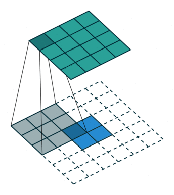
- 將處理後的feature map分別送入幾個dilated rate不同的Atrous Convolution，最後再組合起來(如下圖)，以減少atrous convolution帶來不連續的破碎問題。
- 先downsample再upsample的方式，去做影像分割
- 計算量較少，可是在切割細節上卻沒有辦法表現得很好，因為當output stride是32 (一般classification用的網路多是這個倍率)的時候，圖片中pixel小於32的物件，是沒有辦法被decoder復原回來的
- 本來decode部份在deeplab v3只是bilinear的upsample上去而已，而在v3+加入了與encoder中feature map大小一樣的low level feature

參考：
- [Dilated Convolution(带洞卷积)](https://blog.csdn.net/comeontoto/article/details/79983557)
- [Deeplab v3+](https://medium.com/%E8%BD%89%E8%81%B7%E8%B3%87%E5%B7%A5%E8%BF%B7%E9%80%94%E8%A8%98/deeplab-v3-3a105519a0cf)
- [人人必须要知道的语义分割模型：DeepLabv3+](https://www.zybuluo.com/Team/note/1443524)
# 目標檢測
## Faster-R-CNN
- 將 Segment 的結果先各自畫出 bounding box，然後以一個迴圈，每次合併相似度最高的兩個 box，直到整張圖合併成單一個 box 為止。可預先找出圖中目標可能出現的位置，這些box即為即候選區域（Region Proposal），此方法在R-CNN中稱為Selective Search。
- fast rcnn使用spp結構，SPP Net在普通的CNN結構中加入了ROI池化層（Region of Interest Pooling），使得網絡的輸入圖像可以是任意尺寸的，輸出則不變，同樣是一個固定維數的向量。
- ROI池化層一般跟在卷積層後面，此時網絡的輸入可以是任意尺度的，在SPP layer中每一個pooling的filter會根據輸入調整大小，而SPP的輸出則是固定維數的向量，然後給到全連接FC層。
- faster rcnn加入一個提取邊緣的神經網絡，也就說找到候選框的工作也交給神經網絡來做
- 引入Region Proposal Network(RPN)替代Selective Search
- RPN放在最後一個卷積層的後面並直接訓練得到候選區域

### RPN(Region Proposal Network)簡介：
- 接在Feature map和ROI pooling之間的小全捲積網路
- 建一個神經網絡用於物體分類+框位置的回歸
- 一部分判斷判斷框之中有無包含物體的機率(分類)，另一部分利用回歸判斷框與ground truth的偏差量(offsets)


參考：
- [關於影像辨識，所有你應該知道的深度學習模型](https://medium.com/cubo-ai/%E7%89%A9%E9%AB%94%E5%81%B5%E6%B8%AC-object-detection-740096ec4540)
- [[物件偵測] S1: R-CNN 簡介](https://medium.com/@ywchiu84021121/object-detection-s1-rcnn-%E7%B0%A1%E4%BB%8B-30091ca8ef36)
- [[物件偵測] S2: Fast R-CNN 簡介](https://medium.com/@ywchiu84021121/obeject-detection-s2-fast-rcnn-%E7%B0%A1%E4%BB%8B-40cfe7b5f605)
- [[物件偵測] S3: Faster R-CNN 簡介](https://medium.com/@ywchiu84021121/object-detection-s3-faster-rcnn-%E7%B0%A1%E4%BB%8B-5f37b13ccdd2)
## YOLO
- 架構
- 
- 利用整張圖作為網絡的輸入，直接在圖像的多個位置上回歸出這個位置的目標邊框，以及目標所屬的類別
- 將物體檢測任務當做一個regression問題來處理，使用一個神經網絡，直接從一整張圖像來預測出bounding box的坐標、box中包含物體的置信度和物體的probabilities 。因為YOLO的物體檢測流程是在一個神經網絡裡完成的，所以可以end to end來優化物體檢測性能。
- 
- 速度快，可達real time
- 因為**YOLO v1**卷積層後面是全連接層。和之前滑動窗口方法的目標檢測相比，因為後面是全連接層，可以整合整張圖片的信息，背景識別錯誤率僅為Fast RCNN的一半
- **YOLO v2**增加drop out與batch normalization，取消了全連接層，而是使用anchor box
- Multi-Scale Training
- **YOLO v3**-Darknet-53基底網路-採用RestNet架構，解決梯度問題-使用 FPN 多層級預測架構以提升小物體預測能力(特徵層從單層 13x13 變成了多層 13x13、26x26 和 52x52單層預測 5 種 bounding box 變成每層 3 種 bounding box (共 9 種))

參考：
- [[物件偵測] S4: YOLO v1簡介](https://medium.com/@ywchiu84021121/object-detection-s4-yolo-v1%E7%B0%A1%E4%BB%8B-f3b1c7c91ed)
- [[物件偵測] S5: YOLO v2 簡介](https://medium.com/@ywchiu84021121/object-detection-s5-yolo-v2-%E7%B0%A1%E4%BB%8B-7c160d07e15c)

# 實例分割
## Mask-R-CNN

- 以Faster R-CNN原型，增加了一个分支用於分割任務
- 以一個標準的卷積神經網絡（ResNet50/101）當作主幹網路，作為特徵提取器。
- 將特徵金字塔網絡（FPN）引入主幹網絡，以在多個尺度上更好地表徵目標。以ResNet50/101 5個階段的residual block的Feature map利用插值upsamping後做element-wise的相加。
- 將FPN的輸出進行RPN後再進行ROI Align(而不是ROI Pooling)
- 最後再進行如Faster R-CNN的BBox迴歸及分類與Mask分支進行反卷積（在每一個ROI裡面進行FCN操作）
### ROI Pooling V.S. ROI Align
- ROI Pool的輸入是ROI的坐標和某一層的輸出特徵，不管是ROI Pool還是ROIAlign，目的都是提取輸出特徵圖上該ROI坐標所對應的特徵。
- **ROI Pooling**：
- 由於預選框的位置通常是由模型回歸得到的，一般來講是浮點數，而池化後的特徵圖要求尺寸固定。故ROI Pooling這一操作存在兩次量化的過程。此時的候選框已經和最開始回歸出來的位置有一定的偏差，這個偏差會影響檢測或者分割的準確度，造成不匹配問題（misalignment）。
- 舉例而言：輸入一張800 $\times$ 800的圖片，有一個665 $\times$ 665的框(框中有一隻狗)，經stride為32的特徵提取後，800 $\to$ 25、665 $\to$ 20.78，於是ROI Pooling將其量化為20。接著在Pooling過程中要池化為7 $\times$ 7，故20 $\to$ 2.86，ROI Pooling再次量化為2。可見經兩次量化後將產生明顯誤差(feature map上0.1個像素誤差，在原圖上即為3.2個像素誤差)。
- **ROI Align**：
- 主要想法為取消量化操作，使用雙線性內插的方法獲得坐標為浮點數的像素點上的圖像數值(即利用數學方法近似一個單元的值)，從而將整個特徵聚集過程轉化為一個連續的操作。
- 同樣舉例：在不進行量化的情況下，進行池化的階段中，每一個單元(bin)中規則置入採樣點(例如4個)，這4個點對應的值(浮點數)通過該bin所包含的點插值計算得到，最後對這4個點求均值或最大值作為這個bin的值，然後進行池化操作。

參考：
- [[物件偵測] S9: Mask R-CNN 簡介](https://medium.com/@ywchiu84021121/%E7%89%A9%E4%BB%B6%E5%81%B5%E6%B8%AC-s9-mask-r-cnn-%E7%B0%A1%E4%BB%8B-99370c98de28)
- [[物件偵測] S8: Feature Pyramid Networks 簡介](https://medium.com/@ywchiu84021121/%E7%89%A9%E4%BB%B6%E5%81%B5%E6%B8%AC-s8-feature-pyramid-networks-%E7%B0%A1%E4%BB%8B-99b676245b25)
- [先理解Mask R-CNN的工作原理，然后构建颜色填充器应用](https://www.jiqizhixin.com/articles/Mask_RCNN-tree-master-samples-balloon)
- [Mask R-CNN 論文筆記](https://www.itread01.com/content/1545670085.html)
- [详解 ROI Align 的基本原理和实现细节](https://blog.csdn.net/Bruce_0712/article/details/80287385)
- [三十分钟理解：线性插值，双线性插值Bilinear Interpolation算法](https://blog.csdn.net/xbinworld/article/details/65660665)

## 一些奇怪的名詞
- AP
- mean AP
- pixel accuracy 標記正確的像素佔總像素比例
- IoU
- freq weighted mean IoU 根據每一類出現的頻率對各個類的IoU進行加權求和
- precision
-  -> G統大佬
- Scikit-Learn
- pillow

# 優化方式

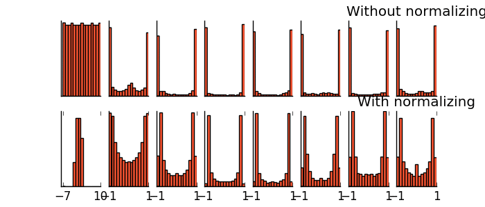
- Batch Normalization(增加準確率與速度)
-- 將每個batch的值做正規化處理
$$
y = \frac{x - \mathrm{E}[x]}{ \sqrt{\mathrm{Var}[x] + \epsilon}} * \gamma + \beta
$$
-- training加速
-- 防止gradient vanishing
-- 幫助 sigmoid 或是 tanh 這種的 activation function
可以讓參數的 initialization 的影響較小
-- 有一些對抗 Overfitting 的效果，但是主要的作用還是用在 training 不好的時候使用，提升 training 的準確率

在tanh上的實現：

- Data Augmentatoin(增加準確率)

## 優化參數

- **Activation Function**

不使用激勵函數的話，神經網絡的每層都只是做線性變換，多層輸入疊加後也還是線性變換。以下三種沒有激勵函數進行平面分割的神經網絡的輸出是線性方程，其用複雜的線性組合來逼近曲線。
明顯線性模型在複雜資料上的表達能力不夠或可能很複雜，因此加入激勵函數以引入非線性因素。
因此激勵函數通常將神經層的輸出進行非線性處理，使最後輸出可以有更多變化。
-- **sigmoid：**
$$\sigma(x) = \frac{1}{1+e^{-x}}$$
其將輸入值映射到介於0~1的值，缺點為當輸入過大或過小時將進入飽和，使梯度消失，且計算涉及自然指數，運算量較大。
-- **tanh：**
$$tanh\ x=\frac{e^{x} - e^{-x}}{e^{x} + e^{-x}}$$
映射至-1~1之間，具zero-centered的特性，但同sigmoid，計算較為繁瑣。
-- **ReLU (Rectified Linear Units)：**
$$f(x) = max(0, x)$$
為線性整流，CNN中常用。對正數原樣輸出，負數直接置零。在正數不飽和，在負數硬飽和。 relu計算上比sigmoid或者tanh更省計算量，因為不用exp，因而收斂較快。但是還是非zero-centered。其中，在負數區域被kill的現象叫做dead relu。

-- **LeakyReLU：**
$$f(x) = max(0.01x, x)$$
讓負數區域不在飽和區死掉。或可將0.01換成可學習的變數$a$，此為**PReLU(parametric rectifier)**。

-- **ELU (Exponential Linear Units)：**
$$f(x) = \left\{ \begin{array} {l} x & \mathrm{if\ x}> \mathrm{0} \\
\alpha (e^x-1) & \mathrm{if\ x \leq 0} \end{array}\right. $$
可以看做是介於relu和LeakyReLU之間的一個東西。當然，這個函數也需要計算自然指數，因此相較計算量上更大一些。

-- **Softmax：**
$$\sigma(z)_i = \frac{e^{z_i}}{\sum_j e^{z_j}}$$
Softmax函數把輸出映射成區間在(0,1)的值，並且做了歸一化，所有輸出的和累加起來等於1。可以直接當作概率對待，選取概率最大的分類作為預測的目標。雖然其中出現指數，但這樣可以讓大的值更大，讓小的更小，增加了區分對比度，學習效率更高。

-- **GELU (Gaussian Error Linerar Units)：**
GELUs對於輸入乘以一個0和1組成的mask，而該mask的生成則是由滿足高斯分布的輸入的機率累積函數(Cumulative distribution function)決定，且滿足伯努利分布(Bernoulli distribution)。即$mask = \Phi(x) = P(X \le x)$，因此：
\begin{align}
GELU(x) &= xP(X \le x) \\
&= \Phi(x) \cdot 1 + (1-\Phi(x)) \cdot 0 \\
&=0.5x\left(1+\text{erf}\left(\frac{x}{\sqrt{2}}\right)\right) \\
&\simeq 0.5x\left(1+\text{tanh}\left(\sqrt{\frac{2}{\pi}}(x+0.044715x^3)\right)\right)
\end{align}
因此當輸入x較小的時候，它將有更高的概率被dropout掉，這樣的激活變換就會依賴於輸入x了。所以GELU可以按當前輸入x比其它輸入大多少來縮放x。

參考：
- [神经网络激活函数汇总（Sigmoid、tanh、ReLU、LeakyReLU、pReLU、ELU、maxout）](https://blog.csdn.net/edogawachia/article/details/80043673)
- [通俗理解神经网络之激励函数(Activation Function)](https://blog.csdn.net/hyman_yx/article/details/51789186)
- [常用激活函数（激励函数）理解与总结](https://blog.csdn.net/qq_45049692/article/details/90266323)
- [神经网络中的Softmax激活函数](https://blog.csdn.net/dcrmg/article/details/79248571)
- [GELU 激活函数](https://blog.csdn.net/liruihongbob/article/details/86510622)
- [超越ReLU却鲜为人知，3年后被挖掘：BERT、GPT-2等都在用的激活函数](https://www.jiqizhixin.com/articles/2019-12-30-4)
- [What is GELU activation? StackExchange](https://datascience.stackexchange.com/questions/49522/what-is-gelu-activation)
- **Loss Function**

在一個模型中，預測值與實際值得落差稱為殘差(residual)。通常會希望損失或殘差最小，也就是使

$$loss\ or\ residual = y - \hat{y}$$

盡可能的越小。其中$y$為預測值，$\hat{y}$為實際值。
-- **平均絕對值誤差(Mean absolute error，MAE)：**
這裡的誤差(error)指的就是殘差。對於分類問題，預測輸出為一組機率，將其減掉實際值有正有負，因此可用絕對值讓差值變成正數。

$$MAE = \frac{1}{n} \sum^n_{i=1}|y - \hat{y}|$$

-- **均方誤差(Mean square error，MSE)：**
由於MAE的梯度始終相同，將使模型權重無法更新至最佳解(在附近來回震盪)，因此使用非線性的MSE。

$$MSE = \frac{1}{n} \sum^n_{i=1} (y - \hat{y})^2$$

解決了MAE的問題，但MSE所計算出的誤差較MAE大了許多，可能造成當資料中出現極大偏差值時權重更新過大，導致模型效果較差。
-- **根均方誤差(Root mean square error，RMSE)：**
為了解決上述問題，對MSE開根號使不同資料的誤差適當縮小但又不失資訊。

$$RMSE = \sqrt{\frac{1}{n} \sum^n_{i=1} (y - \hat{y})^2}$$

-- **交叉熵(Cross-entropy):**
對於一機率函數$p(x)$，首先定義訊息量(information gain)：

$$I(x) = -log_2(p(x))$$

其意義為「一個事件發生的概率越大，不確定性越小，則它所攜帶的信息量就越小」，例如機率為0.5的隨機性的事件比機率為0.99大(更難預測)。至於熵(Entropy，此處特指Shannon Entropy)則表示為系統的亂度或是系統的不確定性，其公式為：

$$H(x) = \sum_i -p_i log_2(p_i)$$

意即熵為所有事件的期望值。因此信息量用來衡量一個事件的不確定度，熵則用來衡量一個系統（也就是所有事件）的不確定度。若為二分類問題，對上式微分可知熵值最大發生在機率均為0.5的情況(如下圖所示)。若熵等於0，也就是說該事件的發生不會導致任何信息量的增加。
基於以上，交叉熵定義為：

$$H = \sum^c_{c=1} \sum^n_{i=1} -y_{c,i}log_2(p_{c,i})$$

其中，$c$是類別數，$y_{c,i}$為獨熱(one hot，此處有的意義)編碼標籤$p_{c,i}$為第$i$筆資料第$c$類別的機率。

參考：
- [機器/深度學習: 基礎介紹-損失函數(loss function)](https://medium.com/@chih.sheng.huang821/%E6%A9%9F%E5%99%A8-%E6%B7%B1%E5%BA%A6%E5%AD%B8%E7%BF%92-%E5%9F%BA%E7%A4%8E%E4%BB%8B%E7%B4%B9-%E6%90%8D%E5%A4%B1%E5%87%BD%E6%95%B8-loss-function-2dcac5ebb6cb)
- [简单谈谈Cross Entropy Loss](https://blog.csdn.net/xg123321123/article/details/80781611)
- [熵与信息增益](https://blog.csdn.net/xg123321123/article/details/52864830)
- [熵 (資訊理論)](https://zh.wikipedia.org/wiki/%E7%86%B5_(%E4%BF%A1%E6%81%AF%E8%AE%BA))

- **Optimizer**

基本算法：
1. 計算目標函數關於當前參數的梯度：$g_t=\nabla f(\omega_t)$
2. 根據歷史梯度計算一階動量和二階動量：$m_t = \phi(g_1,g_2,\cdots,g_t);V_t = \varphi(g_1,g_2,\cdots,g_t)$
3. 計算當前時刻的下降梯度：$\eta_t = \alpha \cdot\frac{m_t}{\sqrt{V_t} + \epsilon}$
4. 根據下降梯度進行更新：$\omega_{t+1}=\omega_t-\eta_t$

$\omega$為待優化參數，$f(\omega)$為目標函數(誤差函數)，$\alpha$為初始學習率，$\epsilon$目的為避免發散並限制更新大小。
-- **SGD (Stochastic gradient descent)**：
在一般的GD中，是一次用**全部**訓練集的數據去計算損失函數的梯度就更新一次參數，而SGD則為一次**跑一個樣本或是小批次(mini-batch)樣本**然後算出一次梯度或是小批次梯度的平均後就更新一次，其改善了GD中內存溢出的問題。缺點為如果學習率太大，容易造成參數更新呈現鋸齒狀的更新，會發生在最後幾步跳不進最佳解。
由於此處不含有動量，因此：
\begin{align}
m_t = \frac{1}{N}\sum_i^Ng_{it} \\
V_t = I^2
\end{align}

帶入3.可得其下降梯度：
$$\eta_t = \alpha \cdot g_t$$

-- **SGD with Momentum(SGDM)**：為了抑制SGD的震盪，SGDM認為梯度下降過程可以加入慣性。下坡的時候，如果發現是陡坡，那就利用慣性跑的快一些。在SGD基礎上引入了一階動量。
$$m_t=\beta_1 \cdot m_{t-1}+(1-\beta_1) \cdot g_t$$

-- **Adagrad**：
其算法是在學習過程中對學習率不斷的調整，這種技巧叫做「學習率衰減(Learning rate decay)」，在一開始會用大的學習率，接著在變小的學習率，以避免在SGD中造成的問題。缺點為在訓練中後段時，由3.可知，可能出現梯度接近0。
$$V_t=\sum^n_{t=1} g_t^2$$

-- **Adadelta/RMSProp**：
由於AdaGrad單調遞減的學習率變化過於激進，我們考慮一個改變二階動量計算方法的策略：不累積全部歷史梯度，而只關注過去一段時間窗口的下降梯度。
$$V_t = \beta_2 \cdot V_{t-1} + (1-\beta_2) \cdot g_t^2$$

-- **Adam (Adaptive Moment Estimation)**：
把SGDM的一階動量和Adadelta的二階動量結合即為Adam。
\begin{align}
m_t &=\beta_1 \cdot m_{t-1}+(1-\beta_1) \cdot g_t \\
V_t &= \beta_2 \cdot V_{t-1} + (1-\beta_2) \cdot g_t^2
\end{align}

$\beta_1$和$\beta_2$分別為一階動量和二階動量的超參數。一般情況下，$\beta_1=0.9,\beta_2=0.99,m_0=0,V_0=0$。另外$m_t$和$V_t$可藉由以下修正以增加在剛開始訓練時的穩定性(參考$\mathrm{An\ intuitive\ understanding\ of\ the\ LAMB\ optimizer}$)：
\begin{align}
\hat{m_t} = \frac{m_t}{1 - \beta_1^t} \\
\hat{V_t} = \frac{V_t}{1 - \beta_2^t}
\end{align}

得到：
\begin{align}
\omega_{t+1} = \omega_t - \alpha \cdot \frac{\hat{m_t}}{\sqrt{\hat{V}_{t}} + \epsilon}
\end{align}
-- **LAMB的先備知識 -- LARS (Layerwise Adaptive Rate Scaling)：**
隨著batch size的增加，每一個epoch所做的迭代數將減少，若要在相同的次數內達到收斂，勢必要增加學習率，然而學習率的增加反而會造成訓練的不穩定(使用暖身(warm up)有一定程度的幫助但仍有機會發散)。因此可以藉由在每一「層」施以不同的學習率以改善此問題：
\begin{align}
\lambda^l = \alpha \cdot \frac{\| \omega^l \|}{\| g_t^l \|}
\end{align}
其中$\lambda^l$為對應第$l$層的學習率，$\frac{\| \omega^l \|}{\| g_t^l \|}$稱為信任率(trust ratio, the ratio between the norm of the layer weights and norm of gradients update)，用來分析訓練時的穩定性。

-- **LAMB (Layer-wise Adaptive Moments optimizer for Batch training)：**
基於具衰減的Adam (AdamW)和LARS的方法，其對於$l$層、$t$時刻的權重更新先定義：
\begin{align}
&r_1 = \| \omega^l_{t} \|
\\ &r_2 = \| \frac{\hat{m}_{t}^l}{\sqrt{\hat{V}_{t}^l + \epsilon }} + \lambda \omega^l_{t} \|
\\ &r = \frac{r_1}{r_2}
\\ &\alpha^l = r \cdot \alpha
\end{align}
其中$r$即為信任率，使用$\sqrt{\hat{V}_{t}^l + \epsilon}$而非$\sqrt{\hat{V}_{t}^l} + \epsilon$的原因為前者能獲得更多資訊(如方向)。因此得到：
\begin{align}
\omega_{t+1}^l = \omega_{t}^l - \alpha^l \cdot (\frac{\hat{m}_{t}^l}{\sqrt{\hat{V}_{t}^l + \epsilon }} + \lambda \omega^l_{t} )
\end{align}
其中$\lambda$為AdamW的超參數。

參考：
- [機器/深度學習-基礎數學(三):梯度最佳解相關算法(gradient descent optimization algorithms)](https://medium.com/@chih.sheng.huang821/%E6%A9%9F%E5%99%A8%E5%AD%B8%E7%BF%92-%E5%9F%BA%E7%A4%8E%E6%95%B8%E5%AD%B8-%E4%B8%89-%E6%A2%AF%E5%BA%A6%E6%9C%80%E4%BD%B3%E8%A7%A3%E7%9B%B8%E9%97%9C%E7%AE%97%E6%B3%95-gradient-descent-optimization-algorithms-b61ed1478bd7)
- [如何理解随机梯度下降（stochastic gradient descent，SGD）？](https://www.zhihu.com/question/264189719)
- [神经网络的优化算法框架](https://blog.csdn.net/ANNILingMo/article/details/80310419)
- [快速神经网络的训练算法LARS/LAMB工作原理 --UC Berkeley在读博士生尤洋](https://blog.csdn.net/weixin_44107973/article/details/94587766)
- [An intuitive understanding of the LAMB optimizer](https://towardsdatascience.com/an-intuitive-understanding-of-the-lamb-optimizer-46f8c0ae4866)
- [LAMB Optimizer for Large Batch Training (TensorFlow version)](https://github.com/ymcui/LAMB_Optimizer_TF)

- **Regularization**
正則化可用來抑制overfit，其方法是在loss function($f(\omega)$)加上限制(constrain，$\lambda$)，使部分的參數歸零(或接近零)。

-- **$L_1$ regularization**
$$f_1(\omega) = f(\omega)+\lambda_1\sum|\omega_i|$$
將其作為新的loss function，取梯度，會得到：
$$\nabla f_1 =
\begin{cases}
\nabla f + \lambda_1, & \text{for $\omega$ > 0} \\
\nabla f - \lambda_1, & \text{for $\omega$ < 0}
\end{cases}
$$
更新參數：
$$\omega_{t+1} =
\begin{cases}
\omega_t - \alpha(\nabla f + \lambda_1), & \text{for $\omega$ > 0} \\
\omega_t + \alpha(\nabla f + \lambda_1), & \text{for $\omega$ < 0}
\end{cases}
$$
可以發現，這樣的操作最終可以使參數歸零。

-- **$L_2$ regularization**
$$f_2(\omega) = f(\omega)+\lambda_2\sum \omega_i^2$$
同樣取梯度，則：
$$\nabla f_2=\nabla f+2\lambda_2 \sum \omega_i$$
得到新參數(為了方便先去除summation)：
\begin{align}
\omega_{t+1} &= \omega_t - \alpha(\nabla f+2\lambda_2 \omega_t) \\
&= (1-2\alpha \lambda_2)\omega_t - \alpha \nabla f
\end{align}
由於$\lambda_2$是一個介於0-1的數，因此這樣的操作可以使參數接近零但不等於零。

### 其他：
- **criterion**
-- CrossEntropyLoss
-- L1Loss
-- MSELoss ...

- **Learning Rate**

- **Batch-size**

## 冷知識

- CNN維度計算 $\begin{align}new_{height} = new_{width} = \frac{(W - F + 1)}{S} \end{align}$

## 有用的資料

- [【Python】TensorFlow學習筆記(二)：初探 TFRecord](https://dotblogs.com.tw/shaynling/2017/11/20/150241)
- [【Python】TensorFlow學習筆記(三)：再探 TFRecord](https://dotblogs.com.tw/shaynling/2017/11/21/162229)