---
tags: ggg, ggg2020, ggg298
---
# GGG 298, jan 2020 - class 1 - NOTES

Titus Brown, [e-mail]
Shannon Joslin, [e-mail]

# Section 1: Binder & R

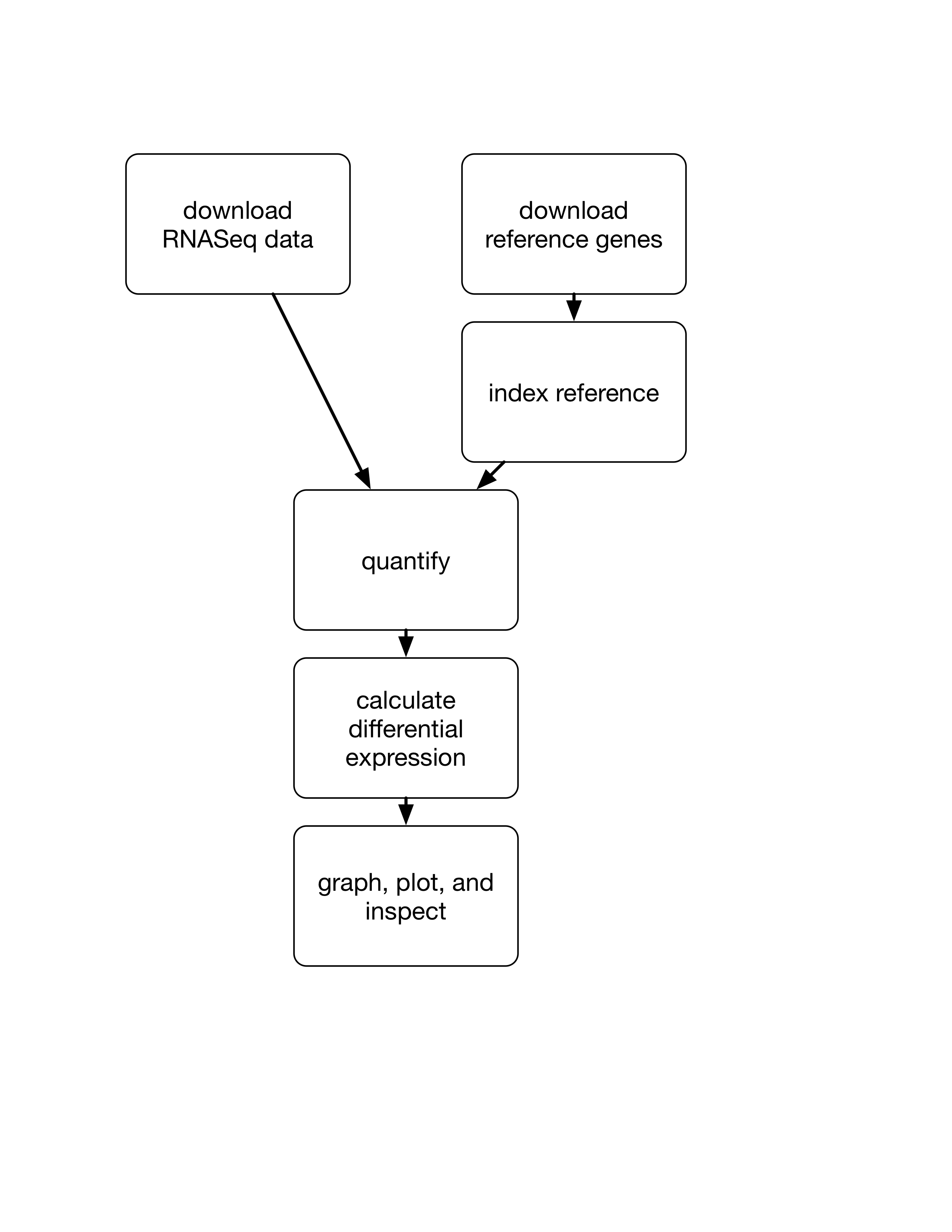
We're going to quickly walk through a first analysis of the data we'll be manipulating this quarter. It's a fairly standard RNAseq analysis, and we won't actually be talking about anything but the commands.

Here's a diagram of what we're going to do:


## Getting started in binder!

Go [here](https://github.com/ngs-docs/2020-ggg-298-first-day-rnaseq) and click on the "launch binder" link at the bottom of the page. This runs RStudio in a ["binder"](https://binder.readthedocs.io/en/latest/user-manual/overview/intro.html), which means you don't need to install anything on your local computer! Here, everything is running in the [Google Cloud](https://cloud.google.com/compute/).

Wait ~10-15 seconds. You should see an RStudio Server window ...sooner or later!

When RStudio has launched, open a Terminal by clicking on the Terminal tab in the top lefthand corner, and copy and paste the commands listed below.

## Configure conda

Do:

conda init
source ~/.bashrc
PS1='$ '

## Install [salmon](https://salmon.readthedocs.io):

Salmon is software to do RNAseq quantification from Illumina short reads. Here we are using [conda](https://angus.readthedocs.io/en/2019/conda_tutorial.html) to install the software. (We'll go through conda in more detail later in the course.)

conda install -c bioconda -y salmon

## Download some data from [Schurch et al, 2016](https://www.ncbi.nlm.nih.gov/pmc/articles/PMC4878611/)

Next, let's download some actual RNAseq data!

I've stored this data on [osf.io](http://osf.io) under a class-specific folder ([here](https://osf.io/vzfc6/)) because it's faster to download from there.

curl -L https://osf.io/5daup/download -o ERR458493.fastq.gz
curl -L https://osf.io/8rvh5/download -o ERR458494.fastq.gz
curl -L https://osf.io/xju4a/download -o ERR458500.fastq.gz
curl -L https://osf.io/nmqe6/download -o ERR458501.fastq.gz

These are [FASTQ files](https://en.wikipedia.org/wiki/FASTQ_format) containing [shotgun Illumina sequencing](https://en.wikipedia.org/wiki/Shotgun_sequencing) of RNA from yeast. You can look at the contents of one of these files like so:

gunzip -c ERR458501.fastq.gz | head

## Download the yeast reference transcriptome:

Salmon needs to know which genes to align the sequencing reads found in the FASTQ files to -- we'll give it the predicted Open Reading Frames (ORFs) from yeast. Download that file:

curl -O https://downloads.yeastgenome.org/sequence/S288C_reference/orf_dna/orf_coding.fasta.gz

Take a look at the contents and compare with the FASTQ reads we downloaded above:

gunzip -c orf_coding.fasta.gz | head

## Index the yeast transcriptome:

In order to work, salmon needs to index the ORFs for a faster search:

salmon index --index yeast_orfs --transcripts orf_coding.fasta.gz

## Run salmon individually on each of the samples:

Let's quantify the number of times each gene in the yeast transcriptome is "hit" by an RNAseq read:

for i in *.fastq.gz
do
   salmon quant -i yeast_orfs --libType U -r $i -o $i.quant --seqBias --gcBias
done

Note here that we're using shell programming (the **for loop**) to write a command that will process _every_ `fastq.gz` file in the folder.

## Collect all of the sample counts using [this Python script](https://github.com/ngs-docs/2018-ggg201b/blob/master/lab6-rnaseq/gather-counts.py):

salmon puts each of the counts in their own directory; gather them all up and rename them so that R can load them more easily.

curl -L -O https://raw.githubusercontent.com/ngs-docs/2018-ggg201b/master/lab6-rnaseq/gather-counts.py
python2 gather-counts.py

## Load in the counts and use edgeR to analyze the samples for differentially expressed genes:

In the RStudio console, copy and paste these lines - note, you can do it one block at a time, if you like.

library("edgeR")

#grab data
files <- c(
"ERR458493.fastq.gz.quant.counts",
"ERR458494.fastq.gz.quant.counts",
"ERR458500.fastq.gz.quant.counts",
"ERR458501.fastq.gz.quant.counts"
)

labels=c("A", "B", "C", "D")

data <- readDGE(files)

print(data)

###

group <- c(rep("mut", 2), rep("wt", 2))

dge = DGEList(counts=data, group=group)
# estimate dispersion
dge <- estimateCommonDisp(dge)
dge <- estimateTagwiseDisp(dge)

## make an MA-plot
# test for diff between 2 groups -binomial counts
et <- exactTest(dge, pair=c("wt", "mut"))
etp <- topTags(et, n=100000)
etp$table$logFC = -etp$table$logFC
# plot global view of the relationship between the expression change between conditions, the average expression strength of the genes, and the ability of the algorithm to detect differential gene expression
pdf("yeast-edgeR-MA-plot.pdf")
plot(
  etp$table$logCPM,
  etp$table$logFC,
  xlim=c(-3, 20), ylim=c(-12, 12), pch=20, cex=.3,
  col = ifelse( etp$table$FDR < .2, "red", "black" ) )
dev.off()

# plot MDS
pdf("yeast-edgeR-MDS.pdf")
plotMDS(dge, labels=labels)
dev.off()

# output CSV for 0-6 hr
write.csv(etp$table, "yeast-edgeR.csv")

## Question: how close is this to a "good" publishing workflow?

What more could/should/would we need to do to make it match an ideal publishing workflow, where we're communicating clearly about the analysis methods?

(Assume no additional *analysis* needs to be done, and we're just talking about communicating what we *did*.)

# Section 2: R Markdown & Beyond
## R Markdown documents!

In order to make our workflow both easy to read by our collaborators and reproducible we can write our workflow in an [R Markdown](https://rmarkdown.rstudio.com/articles_intro.html) document. R Markdown documents contain all of the R code we've used in our console but has the added benefit of producing documents with all of our code and figures.

Let's open up the R Markdown document [RNAseq_Intro.md](https://github.com/ngs-docs/2020-ggg-298-first-day-rnaseq/blob/shannonekj-patch-1/RNAseq_Intro.Rmd) that contains the analysis we've just performed. To do this either click on the RNAseq_intro.Rmd document in the lower right hand corner or click the open an existing file at the top left corner of your RStudio window and select the RNAseq_intro.Rmd file.

Although this document contains the same information that we've just run it looks a little different. R Markdown is a language that allows us to integrate code and comments in one document. Let's see this feature in action by **knitting** our file to generate a document.

Note that we can create a html or pdf depending on which we would like as our final document.

## Creating an R Markdown document from scratch

If you'd like to open a new RMarkdown document in RStudio, click the white square with a green plus sign at the top righthand corner of your RStudio window. Select an "R Markdown..." document.

Once the New R Markdown pane pops up, **fill in the Title and Author** and select to have a default **HTML document**. Then click "OK". At this point an RMarkdown document will open in the top right corner of the RStudio window.

R automatically adds in a lot of information we don't need in our final document but it is useful to remind us of RMarkdown's syntax.

However, you don't have to create your Rmd script in RStudio. You can always write an Rmd document in your favorite text editor!

## Broad advice

Knowledge of data science in general, and sequence analysis in particular, is really useful.

Learn R _**by using it**_.

Learn shell _**by using it**_.

**Participate in the local (and global) community of practice** in data science.

## Other links you might find interesting

UC Davis "stuff":

* [Davis R Users Group](https://d-rug.github.io/) and [Meet and Analyze Data](https://dib-training.readthedocs.io/en/pub/) help groups
* [Data Science Initiative / DataLab](http://dsi.ucdavis.edu/)
* [Data Intensive Biology Summer Institute](http://ivory.idyll.org/dibsi/)