# CNN Note
## Overview
### Jiwon Jeong's article series
Deep Dive into the Computer Vision World: Part 1
- https://towardsdatascience.com/deep-dive-into-the-computer-vision-world-f35cd7349e16
Deep Dive into the Computer Vision World: Part 2
- https://towardsdatascience.com/deep-dive-into-the-computer-vision-world-part-2-7a24efdb1a14
Deep Dive into the Computer Vision World: Part 3
- https://towardsdatascience.com/deep-dive-into-the-computer-vision-world-part-3-abd7fd2c64ef
### An Overview of Early Vision in InceptionV1
https://drafts.distill.pub/circuits-early-overview/?fbclid=IwAR0sF2wJ-nj2PrBjlDd4IauKLdZ0z4UIf_cUJBy6Ttp-yAraiA5N9cfU1-A#mixed3a_discussion_BW

## Concepts
### Output Size of Convolution
- https://towardsdatascience.com/understanding-convolution-neural-networks-the-eli5-way-785330cd1fb7

$$
W_O = \frac{W_I - F + 2P}{S} + 1
$$
$$
H_O = \frac{H_I - F + 2P}{S} + 1
$$
$$
\# outputs = \# input filters
$$
where
- $W_I$ means input width
- $W_O$ means input width
- $H_I$ means input height
- $H_O$ means input height
- $F$ means filter (kernel) size
- $P$ means padding size
- $S$ means the interval at which the filter is appiled
### Type of Convolution Explained
- https://towardsdatascience.com/a-comprehensive-introduction-to-different-types-of-convolutions-in-deep-learning-669281e58215
- https://towardsdatascience.com/types-of-convolutions-in-deep-learning-717013397f4d
- https://github.com/vdumoulin/conv_arithmetic
- https://towardsdatascience.com/types-of-convolution-kernels-simplified-f040cb307c37
#### (Standard) Convolutions
#### Dilated Convolutions
#### Transposed Convolutions
#### Separable Convolutions
- It refers to breaking down the convolution kernel into lower dimension kernels.
- *spatially separable* and *depthwith separable*
#### Spatially Separable Convolutions
<center>A standard 2D convolution kernel</center>

<center>Spatially separable 2D convolution</center>

- not commonly used in deep learning

#### Depthwise Separable Convolutions
<center>A standard 2D convolution with 3 input channels and 128 filters</center>

<center>Depthwise separable 2D convolution which first processes each channel separately and then applies inter-channel convolutions</center>

- widely used and provide really goo performance
- **Efficiency**
- vastly decrease the number of parameters required
#### Deformable Convolutions

- Standard convolutions are very rigid in terms of the shape of feature extraction.
- ***idea: the shape of convolution in itself is learnable***
- implementation
- straightforward
- Every kernel is represented with two different matrics.
- learn to predict the 'offset' of the origin
- simply the convolution branch with input is now the values at these offsets

#### 1x1 convolution related
- https://zhuanlan.zhihu.com/p/40050371
- https://www.zhihu.com/question/56024942
- https://iamaaditya.github.io/2016/03/one-by-one-convolution/
##### outline
- dimension reductionality
- 1x1 Convolution with higher strides leads to even more redution in data by decreasing resolution, while losing very little non-spatially correlated information.
- Replace fully connected layers with 1x1 convolutions as Yann LeCun believes they are the same.
- https://iamaaditya.github.io/2016/03/one-by-one-convolution/

#### Atrous Convolution
- https://towardsdatascience.com/review-deeplabv3-atrous-convolution-semantic-segmentation-6d818bfd1d74
<center>Atrous Convolution with Different Rates r</center>

<center>Atrous Convolution</center>

- For each location $i$ on the output $y$ and a filter $w$, atrous convolution is applied over the input feature map $x$ where the atrous rate $r$ corresponds to the stride with which we sample the input signal.
- This is equivalent to convolving the input $x$ with upsampled filters produced by inserting $r-1$ zeros between two consecutive filter values along each spatial dimension. ("trous" means hold in English)
- When $r = 1$, it is *standard convolution*.
- **By adjusting $r$, we can adaptively modify filter's field-of-view.**
- It is also called **dilated convolution** ([DilatedNet](https://towardsdatascience.com/review-dilated-convolution-semantic-segmentation-9d5a5bd768f5)) or **Hole Algorithm**.
<center>Standard Convolution (Top) Atrous Convolution (Bottom)</center>

- **Top**: Standard convolution.
- **Bottom**: Atrous convolution
- We can see that where $r=2$, the input signal is sampled alternatively.
- First, pad = 2 means we pad 2 zeros at both left and right sides.
- Then, with rate = 2, we sample the input signal every 2 inputs for convoution.
- Atrous convolution **allows us to enlarge the field-of-view of filters to incorporate larger context.
- It therefore offers an efficient mechanism to **control the field-of-view** and **finds the best trade-off between accurate localization (small field-of-view) and context assimilation (large field-of-view)**.

#### involution
https://arxiv.org/abs/2103.06255
https://github.com/d-li14/involution

### NIN
https://towardsdatascience.com/review-nin-network-in-network-image-classification-69e271e499ee

### Loss Functions
Understanding Loss Functions in Computer Vision!
- https://medium.com/ml-cheat-sheet/winning-at-loss-functions-2-important-loss-functions-in-computer-vision-b2b9d293e15a

## Techniques
### im2col
im2col (w/ fancy indexing)
- https://fdsmlhn.github.io/2017/11/02/Understanding%20im2col%20implementation%20in%20Python(numpy%20fancy%20indexing)/
- https://github.com/huyouare/CS231n/blob/master/assignment2/cs231n/im2col.py
- https://hackmd.io/@bouteille/B1Cmns09I
- https://sahnimanas.github.io/post/anatomy-of-a-high-performance-convolution/

### Fast Convolution
- http://people.ece.umn.edu/users/parhi/SLIDES/chap8.pdf

## Arch
### Inception
Deep Learning: Understanding The Inception Module
https://towardsdatascience.com/deep-learning-understand-the-inception-module-56146866e652
<center>naive inception module</center>

<center>A single component of naive inception module. Cost 120M operations</center>

<center>Inception Module Component. Cost only 12M opetaions</center>


Benefits of the Inception Module
* High-performance gain on convolutional neural networks
* Efficient utilisation of computing resource with minimal increase in computation load for the high-performance output of an Inception network.
* Ability to extract features from input data at varying scales through the utilisation of varying convolutional filter sizes.
* 1x1 conv filters learn cross channels patterns, which contributes to the overall feature extractions capabilities of the network.

### Non-Local Blocks
#### Motivations
- https://sh-tsang.medium.com/review-non-local-neural-networks-video-classification-object-detection-segmentation-pose-ac42fe57d0e4
- In videos, **long-range interactions** occur between distant pixels in space as well as time.
- A single non-local block, which is the basic unit, can directly capture these spacetime dependencies in a feedforward fashion.

#### Overview
- https://sh-tsang.medium.com/review-non-local-neural-networks-video-classification-object-detection-segmentation-pose-ac42fe57d0e4
- With a few non-local blocks, the architectures called non-local neural networks are more accurate for video classification than 2D and 3D convolutional networks
- In addition, non-local neural networks are more computationally economical than the 3D convolutional counterparts.
- Self-attention is a special case of non-local operations in the embedded Gaussian version.
- In this work, it gives the insight by relating this recent self-attention model to the classic computer vision method of non-local means.

## Application
### Classification (or Basic Structure)
<center>Adapter from <a href="https://medium.com/yodayoda/segmentation-for-creating-maps-92b8d926cf7e">here</a></center>
#### ResNet
- https://towardsdatascience.com/hitchhikers-guide-to-residual-networks-resnet-in-keras-385ec01ec8ff

#### EffNet
- https://towardsdatascience.com/3-small-but-powerful-convolutional-networks-27ef86faa42d
- Arxiv link: https://arxiv.org/abs/1801.06434
- Use **spatial separable convolution**.

- The separable depthwise convolution is the rectangle colored in blue for EffNet block.
- absence of "normal convolution" at the beginning:

### Object Detection
#### YOLO
- https://allen108108.github.io/blog/2019/11/24/[%E8%AB%96%E6%96%87]%20You%20Only%20Look%20Once%20_%20Unified,%20Real-Time%20Object%20Detection/
- https://towardsdatascience.com/yolo-made-simple-interpreting-the-you-only-look-once-paper-55f72886ab73
- https://towardsdatascience.com/object-detection-with-voice-feedback-yolo-v3-gtts-6ec732dca91

##### source code
- https://medium.com/mlearning-ai/object-detection-explained-yolo-v1-fb4bcd3d87a1

#### YOLOv4
https://towardsdatascience.com/yolo-v4-optimal-speed-accuracy-for-object-detection-79896ed47b50

#### Faster R-CNN
- https://docs.google.com/presentation/d/1SC33WlIT264Ry8cJmqeFyqNZDGMJeQCUAA21a9JOkGM/edit?fbclid=IwAR01L9Nyz1NDhVVQeL89UqSMrxKDIIMwi33YSru3gnB0IHVMBbZJ9XMVQyA#slide=id.p1

#### SSD — Single Shot Detector
- https://towardsdatascience.com/review-ssd-single-shot-detector-object-detection-851a94607d11
- It only need to take **one single shot** to detect multiple objects within the image.
##### Overview
- Three main points
1. Can detect in *multiple scales*.
- With the layers coming after the base network, it yields several feature maps with different resolutions, which enables the network to work at multi-scales.
2. These predictions are made in a convolutional way.
- A set of convolutional filters make the predictions for the location of the objects and the class score.
- This is where the name of "Single Shot" comes from. Instead of having additional classifiers and regressors, now the detections are made in a single shot!
3. There are a fixed number of default boxes associated with these features maps.
- Similar to the anchors of Faster R-CNN, the default boxes are applied at each feature map cell.
##### MultiBox Detector
<center>SSD: Multiple Bounding Boxes for Localization (loc) and Confidence (conf)</center>

- After going through certain of convolutions for feature exteaction, we get **a feature layer of size $m\times n$ (number of locations) with $p$ channels**, such $8\times 8$ and $4\times 4$ above.
- And a $3\times 3$ conv is applied on this $m\times n\times p$ feature layer.
- **For each location, we got $k$ bounding boxes.**
- This $k$ bounding boxes have different sizes and aspect ratios.
- The concept is, maybe a vertical rectangle is more fit for human, and a horizontal rectangle is more fit for car.
- **For each of the bounding box, we will compute $c$ class scores and 4 offsets relative to the original default bounding box shape.**
- Thus, we get **$(c+4)kmn$ outputs.**
- This why the paper is call "SSD: Single Shot **Multibox** Detector"
- But this above it's just a part of SSD.
##### SSD Network Architecture
<center>SSD (Top) vs YOLO (Bottom)</center>

- In order to have more accurate detection, different layers of feature maps are also going through a small $3\times 3$ convolution for object detection as shown above.
- For example, **at Conv4_3, it is of size $38\times 38\times 512$. ($3\times 3$ conv is appiled.)**
- And there are **4 bounding boxes** and **each bounding box will have (classes + 4) outputs.**
- Thus, at Conv4_3, the output is $38\times 38\times 4\times (c+4)$.
- Suppose there are 20 object classes plus one background class, the output will be $38\times 38\times 4\times (21+4)=144,400$.
- **In terms of number of bounding boxes, there are $38\times 38\times 4 = 5776$ bounding boxes.**
- Similarly for other conv layers:
- Conv7: 19×19×6 = 2166 boxes (6 boxes for each location)
- Conv8_2: 10×10×6 = 600 boxes (6 boxes for each location)
- Conv9_2: 5×5×6 = 150 boxes (6 boxes for each location)
- Conv10_2: 3×3×4 = 36 boxes (4 boxes for each location)
- Conv11_2: 1×1×4 = 4 boxes (4 boxes for each location)
- Summing them up we get 5776 + 2166 + 600 + 150 + 36 +4 = **8732 boxes in total**.
- YOLO only gets 7×7×2 = 98 boxes.
- There are 7×7 locations at the end with 2 bounding boxes for each location.
- **SSD has 8732 bounding boxes which is more than that of YOLO.**
##### Loss Function
- The loss function consists of two terms: $L_{conf}$ and $L_{loc}$ where $N$ is the matched default boxes.
<center>Localization Loss</center>

- $L_{loc}$ is the localization loss which is the smooth L1 loss between the predicted box (l) and the ground-truth box (g) parameters.
- These parameters include the offsets for the center point $(c_x, c_y)$, widch ($w$) and height ($h$) of the bounding box.
- Thess loss is similar to the one in Faster R-CNN.
<center>Confidence Loss</center>

- $L_{conf}$ is the confidence loss which is the softmax loss over multiple classes confidence \(c\). ($\alpha$ is set to 1 by cross validation).
- $x_{ij}^p = {1,0}$, is an indicator for matching $i$-th default box to the $j$-th ground truth box of category $p$.
##### Scales Details of Training
<center>Scale of Default Boxes</center>

- Suppoer we have $m$ feature maps for prediction, we cna calculate $s_k$ for the $k$-th feature map.
- $S_{min}$ is 0.2, $S_{max}$ is 0.9.
- That means the scale at the lowest layer is 0.2 and the scale at the highest layer is 0.9.
- For each scale $s_k$ we have 5 non-square aspect ratios:
<center>5 Non-Square Bounding Boxes</center>

- For aspect ratio of 1:1 we get $s_{k}^{'}$:
<center>1 Square Bounding Box</center>

- Hence, we can have at most 6 bounding boxes in total with different aspect ratios.
- For layers with only 4 bounding boxes, $a_r = 1/3$ and 3 are omitted.
##### Some Details of Training
1. Hard Negative Mining
- Instead of using all the negative examples, we sort them using the hightest confidence loss for each default box and pick the top ones so that the ratio between the negatives and positives is at nost 3:1.
- Leads to faster optimization and a more stable training.
2. Data Augmentation
- Each training image is randomly sampled by:
- entire original input image
- sample a patch so that the overlap with objects is 0.1, 0.3, 0.5, 0.7, and 0.9.
- randomly sample a patch
- The **size of each sampled patch is [0.1, 1]** or original image size, and **aspect ratio from 1/2 to 2**.
- After the above steps, each sampled patch will be **resized to fixed size** and maybe **horizontally flipped with probability of 0.5**, in addition to some **photo-metric distortions**.
3. Atrous Convolution (Hole Algorithm / Dilated Convolution)
- The base network is VGG16 with pre-trained weight of ILSVRC classification dataset.
- FC6 and FC7 are **altered to convolution layers as Conv6 and Conv7**.
- Moreover, **FC6 and FC7 use Atrous Convolution**
- And **pool5 is changed from 2×2-s2 to 3×3-s1.**
<center>Atrous convolution / Hole algorithm / Dilated convolution</center>

- As we can see the feature maps are large at Conv6 and Conv7, using Arous Convolution as shown above can **increase the receptive field while keeping number of parameters relatively fewer** compared to conventional convolution.
##### Results
- see here: https://towardsdatascience.com/review-ssd-single-shot-detector-object-detection-851a94607d11

#### FPN (Feature Pyramid Network)
##### Overview

What's the point having this kind of architecture? The information for the precise location of an object can be detected in the deeper level of the network. On the contrary, the semantics gets stronger in the lower level. When a network has one way of just going more in-depth, there aren't many semantic data we can use to classify objects at a pixel level. Therefore by implementing a feature pyramid network, we can produce multi-scale feature maps from all levels, and the features from all levels are semantically strong.
<center>The architecture of FPN</center>

So the architecutre of FPN is shown above. There are three directions, bottom-up, top-down and lateral directions:
* The bottom-up pathway is the feedforward computation of the backbone ConvNet and ResNet as used in the original paper.
* There are 5 stages and the size of the feature map at each stage has a scaling step of 2.
* There are differentiated by their dimensions, and we call them as **C1, C2, C3, C4 and C5**.
* The higher the layer goes, the smaller the size of the feature map gets along the bottom-up pathway.
* Now at the level **C5**, we move to the top-down pathway.
* Upsampling is applied to the output maps at each level. And the corresponding map that has the same spatial sizoe from the bottom-up pathway, is merged via a lateral connection.
* A 1x1 convolution is appiled before the addition to match the depth size.
* Then, we apply a 3x3 convolution on the merged map to reduce aliasing effect of upsampling.
* By doing so, we can combine the low resolution and semantically strong features (from top-down pathway) with high resolution and semantically weak features (from bottom-up pathway).
* This implies we can have rich semantics at all scales. And as shown in the picture, the same process is iterated and produces **P2, P3, P4, and P5**.

Now the last part of the network is an actual classification. Actually, FPN isn't an object detector in itself. A detector isn't *built-in* so we need to plug in a detector from this stage. RPN and Fast R-CNN are used in the original paper, and only FPN with RPN case is depicted in the above picture. In the RPN, there are two sibling layers for an object classifier and bounding box regressor. So in FPN, this part is attached to the tail of each level of **P2, P3, P4 and P5**.

#### RetinaNet
##### Overview
> RetinaNet is **more about proposing a new loss function to handle class imblance**, rather than publising a novel new network.

Let's bring the class imblance back again. One-stage detectors such as SSD and YOLO are apparently faster but still fall behind in accuracy compared to two-stage detectors. And the class imblance issue is one of the reasons for this drawback.
<center>Focal Loss</center>

So the author proposed a new loss function called **focal loss** by putting a weight on easy examples. The mathematical expression is as shown above. It's a cross-entropy loss multiplied with a modulating factor. The modulating factor reduces the impact of easy examples on the loss.

For example, compare the loss when Pₜ= 0.9 and γ = 2. If we say the cross-entropy loss as CE, then the focal loss becomes -0.01CE. The loss becomes 100 times lower. And if the Pₜ gets bigger, say 0.968, with the constant γ, the focal loss becomes -0.001CE (as (1–0.968)² = (0.032)² ≈ 0.001). So it puts down the easy examples even harder and adjusting the imblance in return. And when γ increase, as you can see the graph on the right, the loss gets smaller as the weight increases when Pₜ is constant.

<center>The architecture of RetinaNet</center>

The architecture of RetinaNet is shown above. As we now know ResNet, RPN of faster R-CNN and FPN, there is no nothing new here. The network can be divided into two parts, a backbone with (a) and (b), and two subnets for classification and box regression. The backbone network is composed of ResNet and FPN and the pyramid has levels **P3 to P7**.

As with RPN, there are prior anchor boxes as well. The size of anchors changes according to its level. At the level **P3**, the anchor *area* is 32\*32 and at **P7**, it's 512\*512. The anchors have three different ratios and three different sizes, so the number of anchors of anchors **A** for each level is 9. Therefore, the dimension of output from a box regression subnet is **(N x N) x4A**. And when the number of classes in the dataset is **K**, the output from a classification subnet becomes **(N x N) x KA**.

The result was quite eye-catching. RetinaNet outperformed all the previous networks in both accuracy and speed. RetinaNet-101-500 indicates the network with ResNet-101 and a 500-pixel image scale. Using larger scales gives higher accuracy than all two-stage approaches, while still being fast enough as well.
<center>Speed vs Accuracy on COCO dataset</center>

##### Training and Inference
https://github.com/ramarlina/retinanet-player-ball-detection
https://towardsdatascience.com/detecting-soccer-palyers-and-ball-retinantet-2ab5f997ab2

#### MobileNet
- https://towardsdatascience.com/3-small-but-powerful-convolutional-networks-27ef86faa42d
- Use **depthwise separable convolutions**.
- first introduced by [Xception](https://arxiv.org/abs/1610.02357)

#### MobileNetV2
- https://towardsdatascience.com/mobilenetv2-inverted-residuals-and-linear-bottlenecks-8a4362f4ffd5
##### Inverted Residuals
- Original residual block (ResNet) follows a wide->narrow->wide approach.
<center>A residual block connects wide layers with a skip connection while layers in between are narrow</center>

- On the other hand, MobileNetV2 follows a narrow->wide->narrow approach.
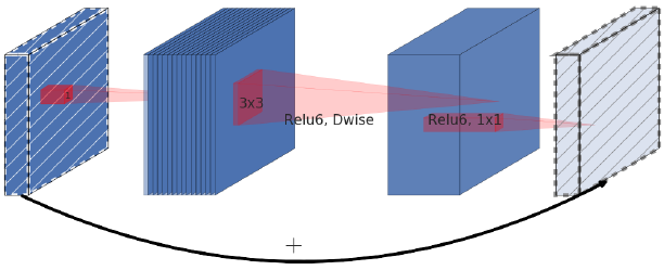
<center>An inverted residual block connects narrow layers with a skip connection while layers in between are wide</center>

- The author describes this idea as an **inverted resudial block** beasue skip connections exist between narrow parts of the network which is opposite of how an original residual connection works.
- The inverted block has **far fewer** parameters.
- With inverted residual block we do the opposite and sqeeze the layers where the skip connections are linked.
- This hurts the performance of the network.
##### Linear Bottlenecks
- The author introduces the idea of a linear bottleneck where the last convolution of a residaul block hasha linear output before it’s added to the initial activations.
- Putting this to code is super simple as we **simply dicard the last activation function** of the convolution block.

##### ReLU6
- omitted as straightforward

#### MobileNetV3
##### Review
- https://towardsdatascience.com/everything-you-need-to-know-about-mobilenetv3-and-its-comparison-with-previous-versions-a5d5e5a6eeaa

#### ShuffleNet
- https://towardsdatascience.com/3-small-but-powerful-convolutional-networks-27ef86faa42d
- Introduce three variants of the Shuffle unit.
- composed of **group convolutions** and **channel shuffles**.

##### Group Convolution
- simply several convolutions with each taking a portion of the input channels.
- In the following picture you can see a group convolution, with 3 groups, each taking one of the 3 input channels.

- First introduce by AlexNet to split a network into two GPUs.

##### Channel Shuffle
- randomly mix the output channels of the group convolutions.
- trick of produce randomness see [here](https://github.com/arthurdouillard/keras-shufflenet/blob/master/shufflenet.py#L37-L48)

#### Metrics
https://github.com/rafaelpadilla/Object-Detection-Metrics

#### Interview Questions
https://medium.com/@akulahemanth/interview-questions-object-detection-9430d7dee763

### Semantic Segmentation
#### Hypercolumn
- https://towardsdatascience.com/review-hypercolumn-instance-segmentation-367180495979

#### Image segmentation in 2020
- https://towardsdatascience.com/image-segmentation-in-2020-756b77fa88fc

### Biomedical Image Segmentation
#### U-Net
- https://towardsdatascience.com/retinal-vasculature-segmentation-with-a-u-net-architecture-d927674cf57b
- https://medium.com/srm-mic/a-gentle-introduction-to-u-net-fc4afd12a893

#### U-Net++
- https://towardsdatascience.com/biomedical-image-segmentation-unet-991d075a3a4b

#### Attention U-Net
- https://towardsdatascience.com/biomedical-image-segmentation-attention-u-net-29b6f0827405

### Instance Segmentation (panoptic segmentation)
#### Mask-RCNN
##### Training on Custom Dataset
- https://towardsdatascience.com/train-custom-dataset-mask-rcnn-6407846598db
- https://github.com/miki998/Custom_Train_MaskRCNN

##### Examples
- https://towardsdatascience.com/webcam-object-detection-with-mask-r-cnn-on-google-colab-b3b012053ed1

## MISC
### 纵览轻量化卷积神经网络：SqueezeNet、MobileNet、ShuffleNet、Xception
- https://www.jiqizhixin.com/articles/2018-01-08-6?fbclid=IwAR1udQ2Bizk074fTaoxRDnavpIDXXjF_k5XYZH9SvUjbfblLw8jLovS6Rfo

### An overview of deep-learning based object-detection algorithms.
- https://medium.com/@fractaldle/brief-overview-on-object-detection-algorithms-ec516929be93

### CNN vs fully-connected network for image processing
- A CNN with $k_x = 1$ and $K(1, 1)=1$ can match the performance of a **fully-connected network**.
- The representatation power of the filtered-activated image is least for $k_x = n_x$ and $K(a, b)=1$ for all a, b.
- Therefore, by tuning hyperparameter $k_x$ we can control the amount of information retained in the filtered-activated image.
- Also, by tuning $K$ to have values different from 1 we can focus on different sections of the image.
- By doing both -- tuning hyperparameter $k_x$ and learning parameter $K$, a CNN is guaranteed to have ***better bias-variance*** characteristics with lower bound performance equal to the performance of a **fully-connected network**.
- This can be improved further by having multiple channels.
- Extending the above discussion, it can be argued that a CNN will outperform a fully-connected network if they have same number of hidden layers with same/similiar structure.
- Nevertheless, this comparison is like comparing apples to oranges.

### ResNets, DenseNets & UNets
- https://medium.com/swlh/resnets-densenets-unets-6bbdbcfdf010