---
robots: index, follow
tags: NCTU, CS, 共筆, 機器學習概論, 荊宇泰, 鄭昌杰
description: 交大資工課程學習筆記
lang: zh-tw
dir: ltr
breaks: true
disqus: hackmd
GA: UA-100433652-1
---
# 機器學習概論--荊宇泰、鄭昌杰
`NCTU` `CS`
[回主頁](https://hackmd.io/s/ByOm-sFue)
建議如果不是想走 AI 的人想要認識 ML 了話可以來修
如果想走 AI 了話,這堂課可能會太淺
# Syllabus
- 前半部: 荊宇泰,介紹為主
- 後半部: 鄭昌杰,偏重數學
- Book: Fundamentals of machine learning for predictive data analytics
- Materials: http://machinelearningbook.com/teaching-materials/
- Language: 不設限,建議用 python, MATLAB
- Grade:
- 期中期末 (占分較重)
- 3 次作業
- 期末專題
- Reference:
- [台大李宏毅教授開的課](http://speech.ee.ntu.edu.tw/~tlkagk/courses_ML16.html)
- 台大林軒田教授開的課
- [機器學習基石](https://www.youtube.com/playlist?list=PLXVfgk9fNX2I7tB6oIINGBmW50rrmFTqf)
- [機器學習技法](https://www.youtube.com/watch?v=A-GxGCCAIrg&list=PLXVfgk9fNX2IQOYPmqjqWsNUFl2kpk1U2)
- CMU Tom Mitchell開的課
- [Video](https://www.youtube.com/watch?v=m4NlfvrRCdg&list=PLAJ0alZrN8rD63LD0FkzKFiFgkOmEtltQ)
- [Lecture Notes](http://www.cs.cmu.edu/~ninamf/courses/601sp15/lectures.shtml)
- [Google dev ML](https://www.youtube.com/watch?v=cKxRvEZd3Mw&index=7&list=PLOU2XLYxmsIIuiBfYad6rFYQU_jL2ryal): Lab 可以參考
- [小遊戲](http://playground.tensorflow.org/?utm_campaign=ai_series_pipeline_051116&utm_source=gdev&utm_medium=yt-desc#activation=tanh&batchSize=10&dataset=spiral®Dataset=reg-plane&learningRate=0.03®ularizationRate=0&noise=0&networkShape=6,2&seed=0.93683&showTestData=false&discretize=false&percTrainData=80&x=true&y=true&xTimesY=true&xSquared=true&ySquared=false&cosX=false&sinX=true&cosY=false&sinY=false&collectStats=false&problem=classification&initZero=false&hideText=false)
# Course
## Ch0~3
### Preface
- What is learning?
- How to learn?
- How to understand?
→ Study language in **math**.
→ Regular Expression & Finite State Automata
→ Memory (Automata, Context-Free)
→ Context sensitive
→ Natual language
- Past:
→ 問題
→ 有解 or 繼續跑 (不知道到底是否要kill掉)
→ 沒希望
- Present:
→問題
→ 不在乎唯一解,只需要學習可能答案、近似值
### Regression Problem(迴歸問題):
- Form: $X_{n\times m}\times M_{m\times l}=Y_{n\times l}$
- Terminology
$$
\begin{equation}
\begin{bmatrix}
x_{11} & x_{12} & x_{13} \\
x_{21} & x_{22} & x_{23} \\
x_{31} & x_{32} & x_{33} \\
\end{bmatrix}
\cdot
\begin{bmatrix}
m_1\\
m_2\\
m_3\\
\end{bmatrix}=
\begin{bmatrix}
y_1\\
y_2\\
y_3\\
\end{bmatrix}
\end{equation}
$$
- Each row in $X$ is called an *instance* ($x_{21} x_{22} x_{23}$)
- Each colcumn in $X$ is called a *feature* $(x_{12} x_{22} x_{23})^T$
>e.g. Gender, Height, Hair Style, Outfit, ...
- $Y$ is called the *target*, each column corresponds to an instance
### Classification Problem
- Classify Instances into different Categories
- See Also: https://en.wikipedia.org/wiki/Support_vector_machine
> e.g. Find a Hyper-Plane that divides K-Dimensional Space points to different regions.

> e.g. MNIST hand-written digit classification:
> https://en.wikipedia.org/wiki/MNIST_database
### Predictive Data Analytics
Predictive data analytics encompasses the business and data processes and computational models that enable a business to make **data-driven decision**
先將 data 分析,得到結論$\to$用來做 decision
- Data Sources
- Data Analytics
- Prediction (Decision) Making
e.g.
- Price Prediction
- Fraud Detection
- Risk Assessment
- Propensity Modelling
- Diagnosis
### Supersived machine learning:
- Requiring Training Dataset (with Label)
- feature
- target
- Use Machine Learning Algorithm
- Model Training
- Prediction Making
- Take Query
- Based on Pretrained Model
- 檢查 *descriptive feature* 和 *target feature* 的關係
- Consistent Prediction Model
```python=
if LOAN-SALARY RATIO > 3 then
OUTCOME = 'repay'
else
OUTCOME = 'default'
```
### How to work
尋找 possible prediction model 集合中最符合
- look for models that are consistent with data
- ill-posed problem: 非唯一解
- Consistency = memorizing the dataset
- Consistency with **noise** in the data isn't desirable
- Goal: generalises and predict
what criteria should use for choosing model
- Inductive bias(訓練規則)
- two types
- restriction (必要的限制)
- preference (偏好)
- searching for potential model
- two source
### Problem
No free lunch
Wrong inductive bias
- Underfitting: Not enough train 訓練不足,得到的結果與真實函式不符
- Overfitting: Overly Trained 訓練過多,得到的結果與真實函式不符
- 符合訓練的dataset
- 在有noice的狀況下,會符合到noise
curve fitting
deep learning like: find all fitting, let algorithm choose the right one
many different types of ML
- Information based: 根據最亂的地方來分
- Similarity based: 定義 feature 到空間中的點的距離(相似度)
- Probability based: 貝式定理
- Error based: 最小化錯誤
### analytic base table (ABT)
\begin{equation}
\begin{bmatrix}
feature1_{for_A} & feature2_{for_A} & ... & featuren_{for_A} \\
feature1_{for_B} & feature2_{for_B} & ... & featuren_{for_B} \\
... \\
feature1_{for_N} & feature2_{for_N} & ... & featuren_{for_N} \\
\end{bmatrix}
\cdot
\begin{bmatrix}
weight_1 \\
weight_2 \\
... \\
weight_n \\
\end{bmatrix}
\end{equation}
### Feature
- raw feature: 原始的資料
- derived feature: 處理過後的資料(除noise, 抓出要的 feature ...)
- e.g. 出生率 - 死亡率 = 人口變化
- continue feature: 連續
- categorized feature: 離散的值
### scatter plot 分布圖
- 可看出 feature 間的 correlation
### 當 data 太多時 $\to$ sampling
- random sampling
- top sampling
- [under sampling](https://en.wikipedia.org/wiki/Undersampling)
- sacrificed sampling
- ...
> 參考
>> [抽樣代表性](http://www.cuhk.edu.hk/soc/lsonline/ies/ies2009/2/electure2_4.htm)
>> [over/under sampling](http://hhtucode.blogspot.tw/2013/08/ml-imbalance-data.html)
>> [MCMC](https://read01.com/zLn6K.html)
ill-posed
- generalize
- inductive bias
- underfitting
- overfitting
- undersampling (欠採樣)
- 練習比較這個人會選交大或清大 XDD
## Ch4 Information base learning
- Decision Tree
可藉著一層一層的問題來尋找結果
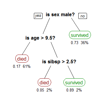
- 特徵選擇、建樹、剪枝
- Information Based
- Figure out which features are the most informative
- Decision tree with:
- root
- interior node
- leaf (terminal node)(outcome)
- 不會整組資料拿去訓練 (To prevent Overfitting)
- Cross Validation
> e.g. 將資料分成 3/4 and 1/4,可能 3/4 拿來 training,1/4 拿來 testing
- shallow tree
- test suspicious words
- descriptive feature split dataset
- entropy
- what is entropy (亂度)
- entropy model defines a computational measure of the impurity of the elements of a set
- uncertainty associated with guessing the result if you were to make a random selection from the set
- high probability -> low entropy
- take the log of probability
- Definition: $H(t) = -\sum_{i=1}^I(P(t=i) * log_2(P(t=i)))$
- more info gain, more easy to used
- Information
- 資訊量是否足夠
- pure subset => entropy low
- $H(t,D) = -\sum(P(t=I)*log_2(P(t=I)))$:亂度
- **亂度即為 $\lg(\frac{1}{p})$ 的期望值**
- remainder (根據資訊分下來的結果)
- $rem(word,D)=\sum(\dfrac{|D_{d=l}|}{|D|}*H(t,D_{d=l}))$:每個partail的亂度加權
- descriptive feature
- information gain $IG(word,D)=H(all,D)-rem(word,D)$: parent亂度減去這種選法的rem
- ID3 Algo (Standard Approach)
- 利用Information Gain選擇node要用的feature
- 資料大時,問題較少
> 使用的資訊獲利會傾向選擇擁有許多不同數值的屬性,例如:若依學生學號(獨一無二的屬性)進行分割,會產生出許多分支,且每一個分支都是很單一的結果,其資訊獲利會最大。
- 建樹
1. using **information gain** choose best descriptive
2. add root node
3. train dataset parition using descriptive
4. for each node
5. precess again **information gain**
- 特徵選擇
1. 算出此node的亂度(parent)
2. 算出要選擇的feature的children的加權亂度
3. 得到此feature的IG
4. 比較每個feature的IG,取IG最大的做這次的節點分類
- 3 situation when recursion stop
- dataset with same classification, return it's classify
- set of features left to test is empty, return major class (如果這箇leaf下還是有多種結果,選結果中最大量的用)
- if empty, return parent classify (如果這條路不曾有過train data,就用parent中最多的答案)
- C4.5
- 用信息增益比率(gain ratio)来作为选择分支的准则
- Gain ratio
$GR(d,D)=\dfrac{IG(d,D)}{-\sum(P(d=l)*log_2(P(d=l)))}$
$GR(D,A)=\frac{IG(D,A)}{SplitInfo(D,A)}$
- 分裂信息(Split information)(IG 以前算的亂度是 target 的, SP 算的亂度是要算得那個 feature 的)
$SplitInfo(D,A)=\sum(\frac{|s+i|}{|S|}\lg{\frac{|s_i|}{|S|}})$
- 複雜度較高
- [CART](http://blog.csdn.net/u011067360/article/details/24871801)
- ID3 優化
- ID3中根据属性值分割数据,之后该特征不会再起作用,这种快速切割的方式会影响算法的准确率
- 每個node只有二分
- 使用Gini作分割
- Gini index(取代 Entropy 來算需要用何 feature 分割)
$Gini(t,D)=1-\sum P(d=l)^2$
- Extensions
- [驗證](http://www.gss.com.tw/index.php/focus/eis/157-eis82/1540-eis82-2)
- using **cross validation** to choose best model (將 data 分成 training 用或 testing 用)
- **k-fold** cross validation:
- 算這個 module/rule 下的平均準確度
- 將資料分為 n 分
- 取一份出來當 testing,剩下的都是 training
- 每次 train 完之後都跟 test 確認精確度
- 精確度平均
- 可得同一 rule 下,不同 training data 的平均精確度
- [cross validation & k-]
- [confusion matrix](http://belleaya.pixnet.net/blog/post/43873939-%5B%E5%AD%B8%E7%BF%92%5D-%5B%E5%88%86%E6%9E%90%5D-%E6%B7%B7%E6%B7%86%E7%9F%A9%E9%99%A3%E8%88%87tp%E3%80%81tn%E3%80%81fp%E3%80%81fn): 用陣列紀錄
$$
\overset{PRIDECT}{
ACTUAL
\begin{bmatrix}
期望A答案A & 期望A答案B & ... & 期望A答案N\\
期望B答案A & 期望B答案B & ... & 期望B答案N\\
...\\
期望N答案A & 期望N答案B & ... & 期望N答案N\\
\end{bmatrix}
}
$$
$$\frac{對角線和}{總和} = 精確度$$
- Problem
- overfitting
- Prepruning(事前修剪noice)
e.g. 限制長度
- Postpruning(事後修剪noice)
e.g. 子樹置換、子樹提升
> Reference
>> http://mropengate.blogspot.tw/2015/06/ai-ch13-2-decision-tree.html
>> http://www.cnblogs.com/wxquare/p/5379970.html
>> http://blog.csdn.net/u011067360/article/details/24871801
### Continuous Descriptive Features
- Process
1. 照 feature sort
2. 每次有 target 改變時設一個 threshold, 值為相加除以二
3. 轉換為分類問題
### Continuous Targets
regression tree (迴歸樹)
- 要讓分完後的 variance(方差) 越小越好
- ${\bf d}[best]=\arg\min_{d \in {\bf d}}\sum(\dfrac{|D_{d=l}|}{|D|}*var(t,D_{d=l}))$
- using ID3 algorithm
- 結束條件不存在全部都一樣的情況
### Noisy Data
在樹越分越細後, noisy 的影響就越加明顯了
- decision tree 較易受影響
### Overfitting((資料)過度使用)
- 樹太深較有可能發生
- feature 多也越容易發生
### Tree Pruning
修剪子樹意謂著利用明顯/平均的target做預測
- Pre-pruning (early stopping criteria)
- 一開始先設好結束條件
- Ex.當樣本數少於5%時結束
- [$\chi^2$pruning](https://en.wikipedia.org/wiki/Chi-squared_test)
- Post-pruning
- 建好樹以後再來拆
- 用測資測測看拆哪裡會有改善
- 用 cross validation 比較剪枝是否會降低準確率, 若不會降低準確率就剪
- Reduced error pruning
用迭代的方式從下到上檢查, 若砍掉 subtree 後的精確度與不砍的相同, 保持砍掉的狀態, 反之將 subtree 接回去
### Model Ensembles
綜合多個 modal 的結果
#### boosting
找到預測錯誤的地方, 對之修正後重建 modal, 將所有 modal 加權
- AdaBoost
建許多 decision tree 並把做錯的 weight 增加, 使得之後建的 decision tree 做對的機率增加
- training data 可能都不同
- iteratively
#### bagging
- sampling with replacement(取後放回)
- subspace sampling
- Random Forest
1. subset sampling
2. ML algo
3. majority voting
- 較易平行化
> reference
>> [Bagging](https://www.youtube.com/watch?v=Rm6s6gmLTdg):
>> 建多個 modal, 選取結果最多的
>
>> [Gradient Boosting](https://www.youtube.com/watch?v=sRktKszFmSk&t=320s):
>> 每次針對錯誤的部分建 modal(正確的點就會消去), 把新建的 modal 加到舊的上
>
>> [Ada Boost](https://www.youtube.com/watch?v=ix6IvwbVpw0):
>> 對預測錯誤的 feature 增加權重, 重建新的 modal, 再將所有 modal 加權
>> [更多 by MIT](https://www.youtube.com/watch?v=UHBmv7qCey4)
## Ch5 Similarity Based Learning
- feature space
- 像是可以定義feature的距離
- similarity metrics(相似性指標)
- distance between instances in feature space
- principle
- **non-negativity**: metric(a,b) >= 0
- **Identity**: $metric(a,b) = 0 \Leftrightarrow a = b$
- **Symmetry**: metric(a,b) = metric(b,a)
- **Triangular Inequality**: metric(a,b) <= metric(a,c) + metric(c,b)
- sample
- $CityBlock(a,b) = |a[i]-b[i]|$
- $Euclidean(a,b) = \sqrt{\sum_{i=1}^m(a[i]-b[i])^2}$(常用)
- $Manhattan(a,b) = \sum_{i=1}^m{abs(a[i]-b[i])}$
- $Minkowski(a,b)= (\sum_{i=1}^m{abs(a[i]-b[i])^p})^{\frac1p}$(p隨modal改變)
### Nearest Neighbor
尋找 query 的 nearest neighbor, 預測 target 與 nearest neighbor 相同
- Voronoi tessellation
- Voronoi region
- decision boundary (將 Voronoi region 圍起來)

### noisy data
- k nearest neighbor
$$M_k(q) = \underset{l\in levels(t)}{\arg\max}\sum_{i=1}^k\delta(t_i,l)$$
- 前 k 個最接近的點 voting
- k 必須是奇數
- k 不能是種類的倍數 (上一點的延伸)
> reference
>> [MIT Open Course](https://www.youtube.com/watch?v=09mb78oiPkA)
>> [ML knn](https://www.youtube.com/watch?v=4ObVzTuFivY)
- weighted k nearest neighbor
- 離散型 target
- weight model (其中一種)
- 前 k 個最接近的點 voting
- 距離越遠的點, voting 的比重越低
$$M_k(q) = \underset{I\in levels(t)}{\arg\max}\sum_{i=1}^k{\frac{1}{dist(q,d_i)^2}*\delta(t_j,l)}$$
- 也有人用高斯分佈做 weight
### data normalize
每個 feature 因為數值的 range 不同, 會造成影響 target 的能力不同 -> 不應該是這樣
- 假設以年齡(歲)跟薪水(元)來分類是否購買, 因為薪水數值>>年齡 => 薪水的影響能力較大 (X)
- 做標準化
$$a_i'=\frac{a_i-\min(a)}{\max(a)-\min(a)}\times(high-low)+low$$
### predict continuous target
- 將最近的 k 個點拿來做平均(knn)
Return $M_k(q)=\frac{1}{k}\sum_{i=1}^kt_i$
- 將最近的 k 個點拿來做漸層(wknn)
$$M_k(q)=\frac{\sum_{i=1}^k{\frac1{dist(q,d_i)^2}}\times t_i}{\sum_{i=1}^k{\frac1{dist(q,d_i)^2}}}$$
### Binary feature
feature 只有二分了話, 是否不用算到 distance 這麼麻煩?
- feature simility
- CP(co-presence): query 跟 sample 都是 true
- CA(co-absence): query 跟 sample 都是 false
- PA(presence-absence): query true 而 sample false
- AP(absence-presence): query false 而 sample true
$$
\begin{array}{c|c c}
n & \text{Query} & \text{Sample} \\
\hline
CP & t & t \\
CA & f & f \\
PA & t & f \\
AP & f & t
\end{array}
$$
- Russel-Rao
- only focus on **CP**
- $sim_{RR}(q,d)=\frac{CP(q,d)}{|q|}$
- e.g. online retail setting (?)
- Sokal-Michener
- focus on **CP** and **CA**
- $sim_{SM}(q,d)=\frac{CP(q,d)+CA(q,d)}{|q|}$
- e.g. medical (是否得病...)
- Jaccard
- sparse data: most of the features have zero values
- $sim_j(q,d) = \frac{CP(q,d)}{CP(q,d)+PA(q,d)+AP(q,d)}$
- e.g. online retail (網路零售 比較使用者看的東西,僅須比較看的東西,沒看的就不用比較)
### Cosine Similarity
- normalized dot product
- feature is **related to each other** (重點在 feature 間的關係)
$sim_{COSINE}(a,b) =
cos(a,b) =
\frac{a\cdot b}{\sqrt{\sum_{i=1}^m{a[i]^2}} \times\sqrt{\sum_{i=1}^m{b[i]^2}}} =
\frac{\sum_{i=1}^m{(a[i]\times b[i])}}{\sqrt{\sum_{i=1}^m{a[i]^2}} \times\sqrt{\sum_{i=1}^m{b[i]^2}}}$
$dist_{COSINE}(a,b)=\frac{\cos^{-1}(sim_{COSINE})}{\pi}$
- [cosine similarity$\approx$Euclidean distance](https://stats.stackexchange.com/questions/146221/is-cosine-similarity-identical-to-l2-normalized-euclidean-distance)
- [also see](http://stackoverflow.com/questions/34144632/using-cosine-distance-with-scikit-learn-kneighborsclassifier)
### [Mahalanobis Distance](https://en.wikipedia.org/wiki/Mahalanobis_distance)
Mahalanobis Distance 在意的是跟 sampling set 之間的關係,尤其是在 sampling set 間若有傾向度(e.g.正/負相關),尤拉距離無法表達出單獨點與整體 set 傾向度間的關係

$$M(a,b) = \sqrt{[(a[1]-b[1]),...,(a[m]-b[m])]\times\sum^{-1}\times\begin{bmatrix} a[1]-b[1] \\ ... \\ a[m] - b[m] \end{bmatrix}}$$
$\sum^{-1}$ 是 **inverse** [covariance matrix](https://zh.wikipedia.org/wiki/%E5%8D%8F%E6%96%B9%E5%B7%AE%E7%9F%A9%E9%98%B5)
$$
CM=
\begin{bmatrix}
cov(feature_1,feature_1) & cov(feature_1,feature_2) & ... & cov(feature_1,feature_n) \\
cov(feature_2,feature_1) & cov(feature_2,feature_2) & ... & cov(feature_2,feature_n) \\
... \\
cov(feature_n,feature_1) & cov(feature_n,feature_2) & ... & cov(feature_n,feature_n) \\
\end{bmatrix}
$$
$cov(a,b)=\frac1{n-1}\sum_{i=1}^n((a_i-\bar{a})\times(b_i-\bar{b}))$,也就是機率中的covelance
觀察,若將 $\sum^{-1}$拿掉,其實就是單純的尤拉距離 => inverse cov matrix 關係到了群集的傾向程度
另一種形式:
$$D^2=(\bf x-m)^TC^{-1}(x-m)$$
\begin{align}
D &= \text{Mahalanobis distance} \\
{\bf x} &= \text{Vector of data} \\
{\bf m} &= \text{Vector of mean values of independent variables} \\
{\bf C^{-1}} &= \text{Inverse Covariance matrix of independent variables} \\
{\bf T} &= \text{Indicates vector should be transposed} \\
\end{align}
- 不應該只考慮 central tendency
- 也可考慮 covariance (協方差)
- 資料分佈不均勻時, 用 Mahalanobis 會比較準確 (Anisotropic 非本向性)
- 考慮到各種特性之間的聯繫
- 尺度無關(scale-invariant)
- Mutual Information
### Efficient Memory Search
- KD tree
- KD tree nearest neighbor retrieval
- descendTree(kdtree, q): find the nearest leaf of the query (從 subtree 找)
- boundaryDist(q,node): if node = leaf, return inf, else return distance between node and q
- parent(node): find the parent of node and delete it(it's leaf)(之後再找subtree時才不會找回原來這棵樹)
- [searching](https://www.youtube.com/watch?v=W94M9D_yXKk&t=15m)
```C++=
找到 query 該放在的 leaf
while 沒有到 root 之上
現在的 node 是否可以更新 best distance? (若則更新)
if query 到 parent [也就是到 boundary] 距離 < best distance
進到 brother 最底(leaf)
else
回到 parent
return best
```
- Other efficient memory search
- sensitivity hashing
- R-Trees
- B-Trees
- M-Trees
- VoRTrees
### Feature Selection
Feature 不是越多越好
data 若不夠多足以支持feature, 反而可能會帶來 noice
$density = {instances}^{\frac{1}{features}}$
- [Curse of Dimensionality](https://zh.wikipedia.org/wiki/%E7%BB%B4%E6%95%B0%E7%81%BE%E9%9A%BE)
維度越高,就需要越多 instance 支持,不然產生稀疏點對,最近點也不足以支持兩者的 target 相近(同)
- type of feature
- *Predictive*
- *Interacting (多個feature一起用)*
- Redundant (多餘的)
- Irrelevant (沒有相關性)
找要用的 feature
- 排名並剪枝 rank and prune (information gain)
- exclude interacting
- include redundant
- greedy local
- Seperate subset of feature
- Forward sequence
- Backward sequence
### [PCA](https://en.wikipedia.org/wiki/Principal_component_analysis)
principal component analysis whth linear algebra
利用 $\lambda$ 做座標轉換
- m features
- n instances
- $n >> m$
- $B$=[ $x_{1}$-$\mu$ | $x_{2}$-$\mu$|...| $x_{n}$-$\mu$ ]
- $S=\frac1{n-1} B\cdot B^{T}$
- 找出 $S$ 的 Eigenvalue($\lambda$)
- 找到最大的eigen value 對應的 eigen vector
- 觀察eigen vector中 不同feature的數值 代表該feature的影響力
經過主軸分析找出m個
...
- data normalize
## Ch6 Probability
- 觀察取樣機率
- $P(A) ← \frac{k}{n}$
- $P(!A) ← 1 - \frac{k}{n}$
- $P(A,B) := P(A \cap B)$
- Condition probility:
- 概念上,條件機率規範了一個機率子空間,所有機率性質在其之上都成立
- $P(A|B) := \frac{P(A\cap B)}{P(B)}$
- $P(A,B) = P(A|B) \times P(B)$
- Bayes' Theorem
- 解讀:
- 機率空間的轉換
- 母空間→條件空間
- 條件空間彼此轉換
- 利用新資訊修改已有看法
- $P(A|B)=\frac{P(B|A)\times P(A)}{P(B)}$
- Beyesian Prediction
- 測試每個分類的機率, 可以利用query的feature與相對的pro算出query的機率
- Conditional Independence and Factorization
- 利用事件在條件空間中的獨立性
- 給定條件空間$C$中獨立的事件序列 $<A_k>$我們有:
- $P(\bigcap_k A_k|C) = \prod_k P(A_k|C)$
- $P(\bigcap_k A_k,C) = \prod P(A_k|C)\times P(C)$
- 名詞
- probability function
- joint probability (多事件)
- conditional proability (條件)
- probability distribution (機率分佈)
$$P(T\ |\ q[1], q[2],...,q[k]) => P(q[1]\ |\ T,q[2],...,q[k])$$
可能可以算的比較快,因為條件T可能可以壓低data
$$P(t=I | q[1],...,q[m]) = \frac{P(q[1],...,q[m] | t=I)P(t=I)}{P(q[1],...,q[m])}(任一項不能等於0)$$
### The Paradox of the False Positive
- 概念:較大的子空間有較小的容錯率
- False Positive:
- 把錯的看成對的
### Bayesian MAP Prediction Model (Maximum a Posteriori)
- 目的:從Feature條件空間下找出最有可能的Target
- 資源:Model已經紀錄各個Target空間的機率分部
- 手段:
- 將Target空間轉換至Feature空間 (Bayes' Theorem)
$$P(target | feature) = \frac{P(feature|target)\times P(target)}{P(feature)}$$
- 選擇Feature空間中機率最大的Target事件作為預測
$$Prediction = arg\max_{target} P(target|feature)$$
- 綜上所述
$$Prediction$$
$$= arg\max_{target} \frac{P(feature|target)\times P(target)}{P(feature)}$$
$$=arg\max_{target} P(feature|target)\times P(target)$$
- Bayesian MAP Prediction Model (without normalization)
### Naïve Bayes' Classifier
- 最大後驗機率估計(MAP)
$$Prediction = arg\max_{target} P(feature|target)\times P(target)$$
- 假設各Target空間中Feature事件彼此**條件獨立** (簡化模型)
$$P(feature|target) = \prod_k P(feature_k|target)$$
- 因此有
$$Prediction = arg\max_{target} \prod_k P(feature_k|target)\times P(target)$$
### Smooth
在算出機率後,如果有些 range 是 0 => $\Pi$ 後會全部變成 0 !!!
為避免產生這種情形,可能空間裡就算 traning data 沒有,也應該要塞機率進去
注意最後機率總和要為1
- Laplacian smoothing
$$P(f=v|t)=\frac{count(f=v|t)+\alpha}{count(f|t)+(\alpha\times Domain(f|t))}$$
- $\alpha$: 改變參數
- Domain(): 對這個 feature 下有幾種分區
- smooth 後整體的趨勢不該改變
### Continous feature
從收集到的資料中,找到一個 function 符合這些資料,之後遇到沒出現過的 feature 時,可以直接用 function 算出結果
- PDF (probability density function)
- 種類
- Normal
- 易受到極端值影響(outline) (極左or極右出現一個雜訊)
- Student-t
- Base function
- 與Normal比較不易受極端值影響
- Exponential
- Mix
- ...
- 誤差
- 採集資料分區的誤差

- 計算
根據target不同做出不同的PDF,query帶入每個PDF算出機率後再使用[Naïve Bayes’ Classifier](#naïve-bayes’-classifier)分析
- e.g.
- 假設決定用 normal distribution 來算:
- 選擇 feature1
- 從 feature1 中再拿出 target1
- 計算這些數字的 平均 & 標準差
- 接著算 feature1 target2 ...
- 以此類推算出 feature_n, target_n
- 這樣就會有 target1 -> feature1, feature2, ... 的平均根標準差
- 利用 PDF 公式 ($f(x) = \frac{e^{-(x - \mu)^{2}/(2\sigma^{2}) }} {\sigma\sqrt{2\pi}}$) 將 testing 的資料丟進去算
- 算法就是算出 target1, target2, ... 的 $\Pi(PDF)$
- 最後找出 $\Pi$ 最大的 target 極為答案
### Continous Feature WITH Binning(切區間)
每個區間該取多大🤔
- equal width
區間用寬度取
- equal frequence (recommand)
區間用頻率取(多少個事件一個區間)
### Bayesian network
Bayesian modual 可以用 network 表示
- DAG(有向無環圖)
- CPT(conditional probability table)
### Markov blanket
要算一個時間點的機率,只要從上一層的機率算就好了,不用算到再之前的 (不用算全部)
$$
P(x_i|x_1,...,x_{i-1},x_{i+1},...,x_n) = \\
P(x_i|parents(x_i))\underset{j\in Children}\Pi P(x_j|parents(x_j))
$$

- 公式證明
(回去再研究 XD)
- 如何建網路: 看資料,but 怎麼建答案都一樣 (應該是差在計算複雜度)
### Markov Chain Monte Carlo(MCMC)
- Monte Carlo
- 針對一個問題,只要取樣夠多夠平均就可以
- Markov Chain
- 要看一個事件,只要看他的前一個狀態(時期)就可以滿足 MarkovChain
- 可變成線性代數模型,矩陣相乘 => 穩定 (矩陣須符合一些規則)
- Hidden Markov Chain
- 沒有轉移矩陣,不知道狀態轉移的方式,但有其他間接方式可以觀察到資訊(Deep Learning 常用)
### Gibbs sampling
(聽不太懂)好像是利用MCMC的性質模擬資料
## Ch7 Error base learning
常用在 Regression
- idea
- y = mx + b, 想尋找符合 sample 的方程式 => 試線性
- 線性夠嗎?
- 想找出一個方程式,使得誤差最小
- $M_w(d)=w[0]+w[1]*d[1]$
- 如何定義誤差
- $L_2(M_w,D)=\frac{1}{2}\sum_{i=1}^n(t_i-M_w(di[1]))^2$
- 真實質與modal值得平方差
- Gradient Distance
$$M_w(d) = \sum_{j=0}^mw[j]\times d[j] = w\cdot d$$
- Convex
- 範圍內只有一個 local minima
- 希望誤差最小
$L_2(M,D)=\frac1 2\sum_{i=1}^n(t_i-M(d_i[1]))^2$
(1/2 是為了之後微分用)
- $t_i$ 是第 i 個事件的 target
### Multivariate Linear Regression with Gradient Descent
$M_w(d)=w[0]*d[0]+w[1]*d[1]+...+w[n]*d[n]\ (d[0] = 1)$
$=\sum_{i=1}^nw[i]*d[i]=w\cdot d$
- 現在有了錯誤方程式,我們需要找最低點,先猜一個點,對此點作偏微分,會得到空間中的斜率,便可以以此作為依據,將點更正到較低點的地方,以此遞迴
- 尋找過程不會是平滑的,而會是震盪的
- 斜率越大,修正距離越大
- 算法條件
- training instances D
- learning rate $\alpha$: 控制斜率與修正變動量的關係
- errorDelta function: 用斜率或其他方法檢查該移動的方向
- 可能方別對每個維度做更新
- 也可以每次都算一個總斜率方向做更正 (weight有相依性的話就要用這個)
- convergence criterion: 終止條件 (可能是成功,也可能是達到了**預期做不到**的條件)
```=pheudocode
w ← random starting point in the weight space // 起點
repeat
for each w[j] in w do // 對每個維度做移動
w[j] ← w[j] + α × errorDelta(D, w[j]) // 原位置+需要更新的長度
end for
until convergence occurs
```

### Gauss-Newton Algorithm
另外一種調教 w 的方法 -> 其實就是 Grandient Descent
- 利用泰勒展開式推得
$f(u)≈ f(u_s)+∆u^Τ f'(u_s)+...$
...
### Linear Regression
判斷 feature 的 weight
- Statistical significance test
- t-test
- 假設一個 instance,用 null hypothesis 來反證
- 假設某 feature 不重要,計算 t-value
- $t=\frac{Z}{s}=\frac{w[j]}{se(d[j])}$
- $se(d[j])=\frac{se}{\sqrt{\sum(d[j]-\overline{d[j]})^2}}$
- 算出 t 後[查表](http://www.socscistatistics.com/pvalues/tdistribution.aspx)
- 雙邊考量
- 也可以評估 data 是否是錯誤 / 亂填的
### weight decay
- Learngin rate decay(衰減)
- $\alpha_\tau=\alpha_0\frac{c}{c+\tau}$
- 調整 c 做出比較好的收斂
### Descriptive Feature
regression 比較適用在 continuous
竟量讓離散的 feature 數值化 => 連續化
- e.g. 有一個欄位負責填 A or B or C
- 將這個欄位拉開來成為 isA, isB, isC 三個欄位
- 每個欄位的值都是 0~1 (有無)
- cons: feature 會變多
### Categorical Target(Logistic Regression)
- target 二分
- boundary 不是 continous 不能作微分
...
### Non-linear Relationship
### SVM
> Data 最好先 normalize
找一條線切開面上的兩個群,且**離兩個群的距離相同(越遠越好)**

- 虛線與實線的距離越遠越好
- $w_0 + \vec{w}\cdot \vec{d} = h$
- 同除 h => $w_0 + \vec{w}\cdot \vec{d} = \pm 1$
- $M_{\alpha,w_o}(q) = \sum_{i=1}^s(t_i\times \alpha[i]\times (d_i\cdot q)+w_0)$
- SVM 只要看 $t_i\times (w_0 + w\cdot d) >= 1$
- $dist(d)=\frac{w_0+abs(w\cdot d)}{|w|}$
- 最終目標:
- 最大化 $\frac2{|w|}$
- subject to the constraint
$t_i\times (w_0 + w\cdot d) >= 1$
#### Lagrange Multiplier Method
在滿足*某個條件*下,找到 local min/max
### 非線性分割
SVM 也可以處理非線性分割
- Basis functions
- $t_i\times(w_0+w\cdot\phi(d))>=1$ for all i
- 把非線性分割 data 丟入一組 basis functions => 將原來的 dataset 轉換到線性分割的資料
- e.g. sklearn.svm.svm(kernel='')
- linear kernel
- $kernel(d, q) = d\cdot q + c$
- polynomial kernel
- $kernel(d, q)=(d\cdot q+1)^p$
- gaussian radial basis kernel
- $kernel(d, q)=exp(-\gamma||d-q||^2)$
- $\gamma$: manually chosen tuning parameter
- ...
## Ch8 ML for Predictive data analytics
> classification: 類別確定好了的分類
> clustering: 類別沒有確定好

### 取樣正確性
- binary prediction
- true positive (TP)
- true negative (TN)
- false positive (FP)
- false negative (FN)
- Confusion matrix
- misclassification accuracy(誤判機率) = $\frac{(FP+FN)}{(TP+TN+FP+FN)}$
- 3 份 data
- training data
- validation data 調參數用
- test data
- k-ford
### 效能評估
- TP/TN/FP/FN R: 比率
- TPR: $\frac{TP}{(TP+FN)}$ (分母都是事實上是對的)
- TNR: $\frac{TN}{(TN+FP)}$
- FPR: $\frac{FP}{(TN+FP)}$
- FNR: $\frac{FN}{(TP+FN)}$
- precision(準確率): $\frac{TP}{(TP+FN)}$
- recall(可信度): $\frac{TP}{(TP+FN)}$
- $F_1-measure$: $2\times\frac{(precision\times recall)}{(precision+recall)}$
-----
## 宇泰小品
如 O(n) 何切 knn 範圍(propossing)
...
Feature
- 注重哪些 feature: 將 N Dimantion 投影到 那幾個 feature 的 space
- Range Query: 把範圍內的所有點取出來
- $\Theta(n)$
- 希望利用 preprossing 將 query 的 $\theta$ 壓下去
- 也可能原來的 domain map 到新的 domain (SVM)
- e.g. $x^2+y^2<r^2$ => $x^2+y^2-r^2<0$
- Range tree
- $O(2\lg(n))$
- 用 x feature 建立出 range tree
- 在每個 node 下掛上這個 x range 下的所有可能 y feature
- kdTree
- 保證 space $O(n\lg(n))$
- time 會花比較長一點的時間 $O(\sqrt{n})$
$U_2(m)=U_2(m-1)+U_3(m-1)+1$
$U_3(m)=2U_3(m-1)+3$
- 從 root 開始往下走,report 在 query 內的點
\可能寫 GPU programming ㄟ/
---
# Lab
~~助教:下面很久沒更新囉~~
## Lab1
- [spec](https://drive.google.com/open?id=16rqNLAnvz21gy0rQItbpKBXseJOryF21U33q4ZEM_ew)
- http://archive.ics.uci.edu/ml/datasets/Iris
## Lab2
- [spec](https://drive.google.com/open?id=0B0YxeEDDLL8XQ2wwOTNuQVA2U0k)
- [教學](https://goo.gl/V6GQl1)
## Lab3
- [spec](https://drive.google.com/open?id=1hPy_tdT3zqgoR0CXN2iW54VhMjFROIS78lvKcKwGtuc)
- [教學](https://goo.gl/cG5tUW)
# Exam
- 4/11
- ch6 前半部 (6A)
# Final Project
### jupyter 視覺化
- using
- pandas
- numpy
- sk-learn (scikit learn)
- matplotlib
- .discript()
- .groupby
- .mean()
- .count
- .subplots(kind=)
- .plot(kind=)
 Sign in with Wallet


