---
tags: BMMB554-23
---

# Lecture 25: Finding matches quickly
> Based on the [course](http://www.langmead-lab.org/teaching-materials/) taught by Ben Langmead at Johns Hopkins. The cover image is from [Wikpedia article](https://en.wikipedia.org/wiki/Burrows%E2%80%93Wheeler_transform) on Burrows-Wheeler transform.
## The challenge of really large datasets
You have a lot of reads and you need to align them against the genome. You can use classical alignment approaches based on the dynamic programming logic (which we will discuss in the next lecture). It will work, but the performance of these approaches expressed as the [big O notation](https://en.wikipedia.org/wiki/Big_O_notation) is:
$\mathcal{O}(mn)$
where $n$ is the read length and $m$ is the genome length. $m$ can be **very** large. For instance, in the case of human genome it is $3\times10^9$. On top of that we *very many* reads. The latest Illumina NovaSeq 6000 machine can produce as much as 20 billion 150 bp eads. Taking this into account our big O notation becomes:
$\mathcal{O}(dmn)$
where $d\times m\times n = 9\times10^{21}$ ($d$ stands for *depth* approximated as read number). In other words to compute alignments between a genome and all these reads we need to perform $9\times10^{21}$ cell updates in the dynamic programming matrices even before we start the traceback. On a cluster containing 1,000 3GHz CPUs this will take over **8** years!
## Mapping versus alignment
One possible idea on how to speed things up will be to first find most likely locations for each read and them refine alignments as necessary. In other words reads should be *mapped* by identifying regions of the genomes from which they most likely originate. The term *mapping* is sometimes used interchangeably with the word "alignment". Yet *mapping* and *alignment* are somewhat different concepts. [Heng Li](http://lh3lh3.users.sourceforge.net/) defines them this way:
* **Mapping**: assigning a sequencing read to a location within genome. Mapping is said to be correct and it overlaps the true region from which this read has originated.
* **Alignment**: detailed placement of every base within a read to a corresponding base within the genome. Alignment is said to be correct is every base if placed correctly.
So let's see how we can find potential read locations quickly. Below is a list of key publications highlighting basic principles of current mapping tools:
* 2009 | How to map billions of short reads onto genomes? - [Trapnell & Salzberg](http://www.nature.com/nbt/journal/v27/n5/full/nbt0509-455.html)
* 2009 | Bowtie 1 - [Langmead et al.](http://genomebiology.com/content/10/3/R25)
* 2012 | Bowtie 2 - [Langmead and Salzberg](http://www.nature.com/nmeth/journal/v9/n4/full/nmeth.1923.htm)
* 2009 | BWA - [Li and Durbin](http://bioinformatics.oxfordjournals.org/content/25/14/1754.long)
* 2010 | BWA - [Li and Durbin](http://bioinformatics.oxfordjournals.org/content/26/5/589)
* 2013 | BWA-MEM - [Li](http://arxiv.org/abs/1303.3997)
* 2014 | Johns Hopkins Computational Genomics Course - [Langmead](http://www.langmead-lab.org/teaching-materials/)
### Indexing and substrings
Indexing is not a new idea. Most books have an index where a word is *mapped* back to a page where it is found. This particular type of index is called *inverted index*. The word *inverted* implies that there is also a non-inverted or *forward* index. The image below explain the distinction between the two:
-----
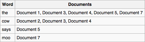
Inverted index

Forward index. (From [Wikipedia](https://en.wikipedia.org/wiki/Search_engine_indexing))
-----
For what we are interested in (searching for the best location of a read in the reference genome) we will use *inverted index*. We will refer to it simply as *index*. So to find a pattern in a string using an index we first need to create that index. To create an index for a string *T* (i.e., a genome) we will need to:
* extract substrings of length *L* and record where these substrings occur;
* organize the list of substrings and their coordinates and an easily accessible data structure (a *map*).
------
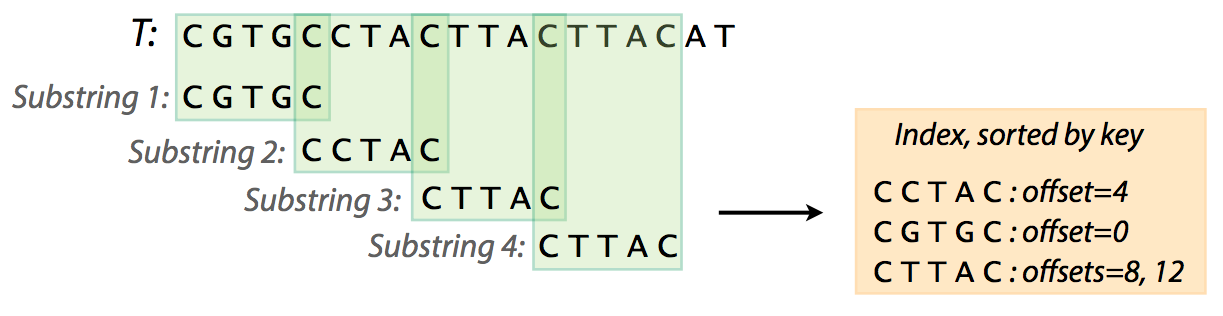
Creating an index. From [Ben Langmead](http://www.cs.jhu.edu/~langmea/resources/lecture_notes/indexing_with_substrings.pdf)
-----
Now that we've created an index for text *T* = `CGTGCCTACTTACTTACAT` we might as well search it. Suppose we now want to find whether a pattern `CTACTTAC` (we will refer to pattern as to *P*) is present in *T*. To do this we need:
* extract substrings from *P*;
* check the index to see if they are present;
* if they are present extend to see if the entire string is matching.
-----
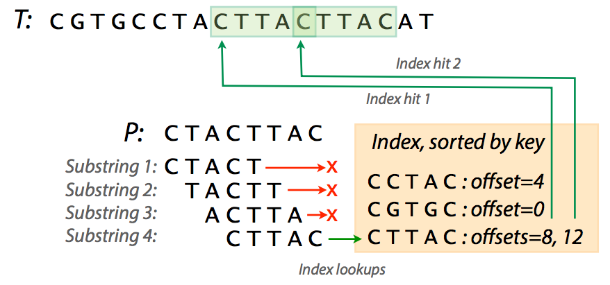
Looking for *P* in *T*. The first three substrings don't have a match. Image from [Ben Langmead](http://www.cs.jhu.edu/~langmea/resources/lecture_notes/indexing_with_substrings.pdf).
----
In the figure above you can see that trying various substrings from *P* yields three failures and a success with two hits. Of course in our case the *T* is very short and you can easily see that an index for a realistic fragment of DNA can be very large. For example, an index for human chromosome 1 (~249,000,000 nucleotides) will occupy over 12 GB of space. In these cases a practical solution may be skipping some of the substrings while making the index. For instance, including only every 4th substring (i.e., using interval of *4*) in a human chromosome 1 index will reduce memory usage to a peak of ~8Gb.
As one can see finding patterns in text using indexes requires finding values for parameters such as substring length and the interval (if we use skipping). These value have significant implications to the speed of the search, memory use, and , importantly, to specificity. The following table shows how choosing different values for substring length and interval affect speed, memory footprint, and specificity for finding pattern `GCGCGGTGGCTCACGCCTGTAATCCCAGCACTTTGGGAGGCCGAGGCGGG`
within human chromosome 1 (data from [here](http://www.cs.jhu.edu/~langmea/resources/lecture_notes/indexing_with_substrings.pdf)):
Substring length | Interval | Indexing time (s) | Search time (s) | Memory usage (Gb) | Specificity (%)
----------------:|---------:|--------------:|------------:|-------------:|-----------:
4 | 4 | 59.31 | 0.40 | ~7.6 | 0.12
7 | 7 | 63.74 | 0.06 | ~5.0 | 1.26
10 | 10 | 72.52 | 0.02 | ~3.6 | 4.11
18 | 18 | 40.20 | 0.02 | ~2.1 | 4.37
30 | 30 | 19.78 | 0.00 | ~1.6 | 11.72
Specificity can be thought of as a proxy for the number of times an index hit can be extended to a true match between *T* and *P*. The figure below explain this idea:
----
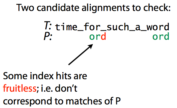
Specificity. Matching `ord` to `time_for_such_a_word`. Image from [Ben Langmead](http://www.cs.jhu.edu/~langmea/resources/lecture_notes/indexing_with_substrings.pdf)
----
here we look for pattern `ord` within text `time_for_such_a_word`. The first index hit does not produce a match, while the second does. Decreasing the number of fruitless hits increases specificity and speeds up the search. Intuitively, this is achieved by increasing the substring length.
In summary, we have seen that we can create an index (a map) containing coordinates of substrings from a text *T*. We can then use this map to find occurrences (if they exist) of pattern *P* within the *T*. The map can be represented in variety of ways including sorted lists, hash tables, and trees:
-----
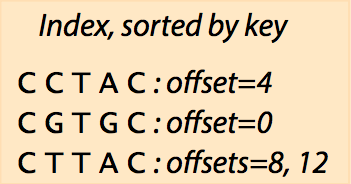
Sorted list
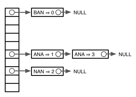
Hash for word `banana`
Trie
Sorted list (top), Hash (middle), and Trie (bottom). From [Ben Langmead](http://www.cs.jhu.edu/~langmea/resources/lecture_notes/indexing_with_substrings.pdf) and [Wikipedia](https://en.wikipedia.org/wiki/Trie#/media/File:Trie_example.svg).
----
What's important here is that sorted lists and especially hash tables provide a quick way to find the initial hit, but they are limited by the choice of the substring size. We've seen before (the *Specificity* table above) that the choice of substring size will have profound effects on the performance of the search. Would it be nice if we would not need to make that choice. For this we will continue to *Tries and Trees* below.
### Tries and trees
Let's consider text *T* = `gtccacctagtaccatttgt`. Using the logic from previous section we can build an index using substrings of length 2 with interval 2 (skipping every other substring) that would look like this after sorting:
| Substring | Offset |
|:---------:|:-------:|
| `ac` | 4 |
| `ag` | 8 |
| `at` | 14 |
| `cc` | 12 |
| `cc` | 2 |
| `ct` | 6 |
| `gt` | 18 |
| `gt` | 0 |
| `ta` | 10 |
| `tt` | 16 |
Representing this sorted list as a *trie* that would map substrings to their positions (offsets) will look like this:
----
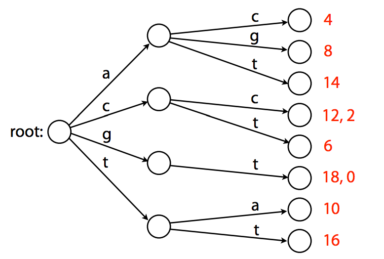
A trie. Example from [Ben Langmead](http://www.cs.jhu.edu/~langmea/resources/lecture_notes/indexing_with_substrings.pdf).
----
Note that this *trie* is the smallest tree ([*trie* versus *tree*](http://stackoverflow.com/questions/4737904/difference-between-tries-and-trees) is indeed a bit confusing) representing a collection of substrings that has the following properties:
* Each edge is labeled with a character from a given alphabet (in this case `A`, `C`, `G`, and `T`);
* Each node has a single outgoing edge corresponding to an alphabet character;
* Each *key* (substrings of length 2 in the above case) is spelled out along a path starting at the root.
While the above example shows how we can quickly find positions for a given substring, it still relies on a fixed substring length. To see how we can deal with this limitation let's introduce the idea of indexing with *suffixes* rather than with fixed substrings. Consider the following text *T* = `GTTATAGCTGATCGCGGCGTAGCGG`. Let's add a special symbol `$` to the end of this text. For *T$* a list of all substrings will look like this:
```
GTTATAGCTGATCGCGGCGTAGCGG$
TTATAGCTGATCGCGGCGTAGCGG$
TATAGCTGATCGCGGCGTAGCGG$
ATAGCTGATCGCGGCGTAGCGG$
TAGCTGATCGCGGCGTAGCGG$
AGCTGATCGCGGCGTAGCGG$
GCTGATCGCGGCGTAGCGG$
CTGATCGCGGCGTAGCGG$
TGATCGCGGCGTAGCGG$
GATCGCGGCGTAGCGG$
ATCGCGGCGTAGCGG$
TCGCGGCGTAGCGG$
CGCGGCGTAGCGG$
GCGGCGTAGCGG$
CGGCGTAGCGG$
GGCGTAGCGG$
GCGTAGCGG$
CGTAGCGG$
GTAGCGG$
TAGCGG$
AGCGG$
GCGG$
CGG$
GG$
G$
$
```
Recall that a trie has the following properties:
* Each edge is labeled with a character from a given alphabet;
* Each node has a single outgoing edge corresponding to an alphabet character;
* Each substring (in this case a suffix) is spelled out along a path starting at the root.
Let's now use these rules to build a suffix trie for a much simpler text *T* = `abaaba`. It is much smaller than the text we used above and so it will be easier to get the point across. First, let's add `$` and create a list of all suffixes:
```
abaaba$
baaba$
aaba$
aba$
ba$
a$
$
```
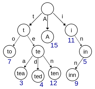
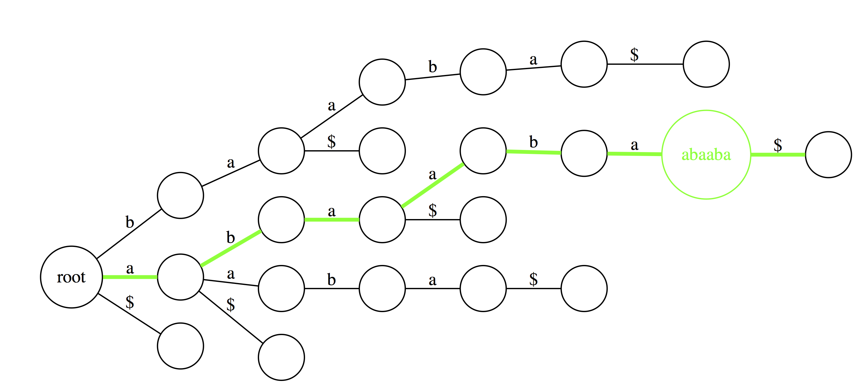
now let's create a trie:
### Looking for substrings in a Trie
----
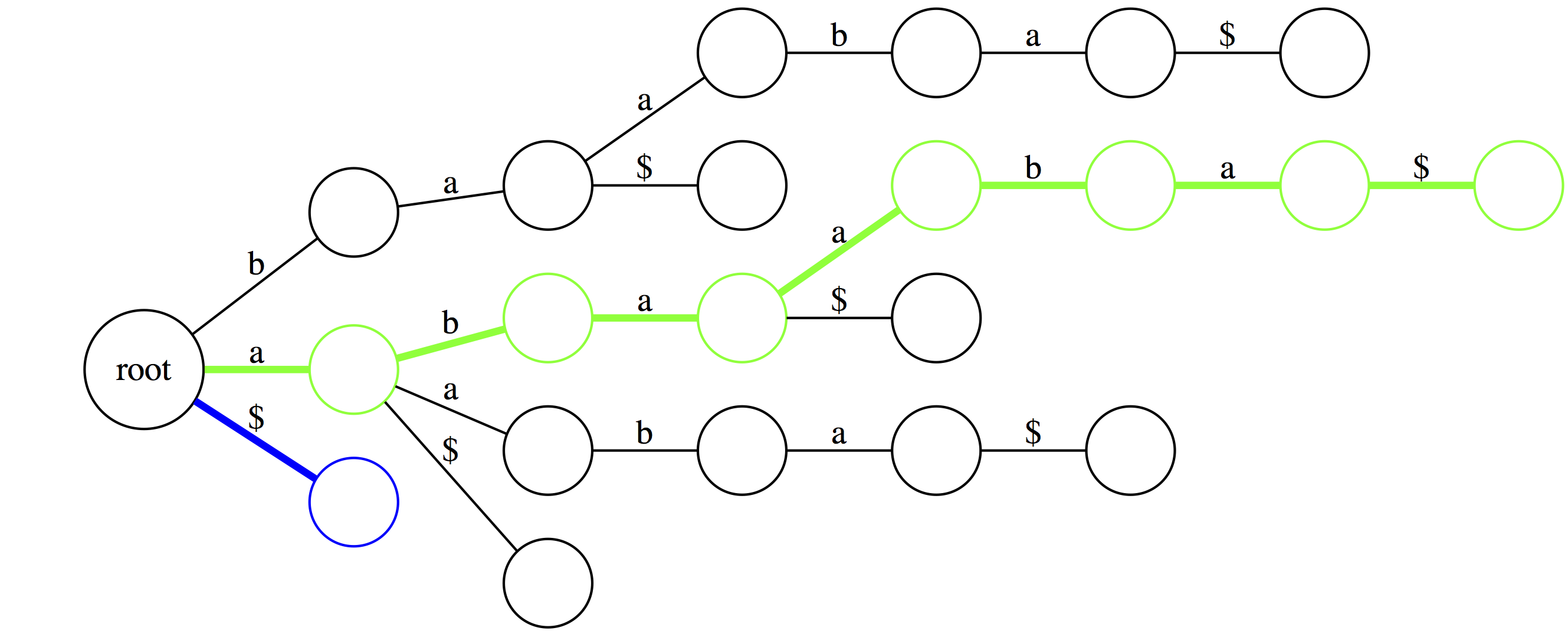
The green path shows the longest suffix (the entire thing). The blue path is the shortest suffix containing only the terminal character.
Note, that the trie would look **dramatically** different had we not added the `$` at the end. The difference is that without the `$` the trie will **not** have every suffix to be represented by a path from `root` to a leaf.
In suffix trie every edge is labeled with a single character and nodes have no labels in our representation. However, you can think of every node as being labeled with a string that spells out all characters occurring along a path from the root up to the that node. For example, the blue node `baa` spells out characters `b`, `a`, and `a` along a path from the root.
Suffix trie is an ideal data stricture to quickly check if a pattern is or is not present in a text. The following three examples highlight how this can be done. Suppose we want to check if a substring `baa` is present within text `abaaba` represented as our suffix trie. We start at the root and take an edge labeled with `b`. We next proceed through an edge labeled `a`. At this point there are two outgoing edges: `a` and `$`. Since the last character in `baa` is `a` we take the edge labeled as `a`. Because the entire substring `baa` can be spelled out as a path from the root we conclude that `baa` is indeed a substring of `abaaba`.
Now let's do the same for `abaaba`. Proceeding along the green path spells out all characters. Again, we conclude that `abaaba` is valid substring.
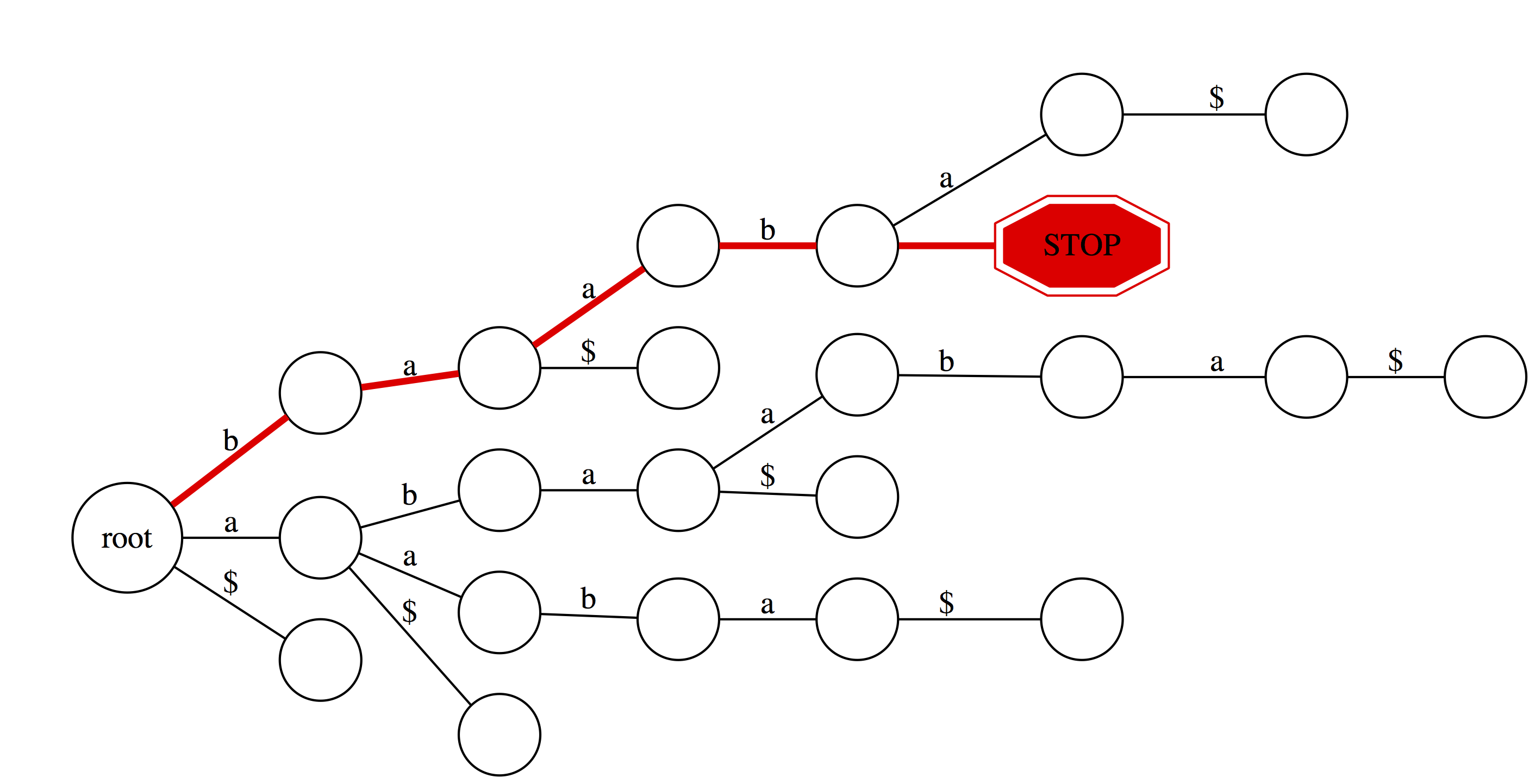
But for `baabb` things look different. We proceed successfully (red path) through `b`, `a`, `a`, and `b`. However, there is no edge labeled `b` at `baab` node. Thus we fall off and conclude that `baabb` is **not** a substring of `abaaba`.
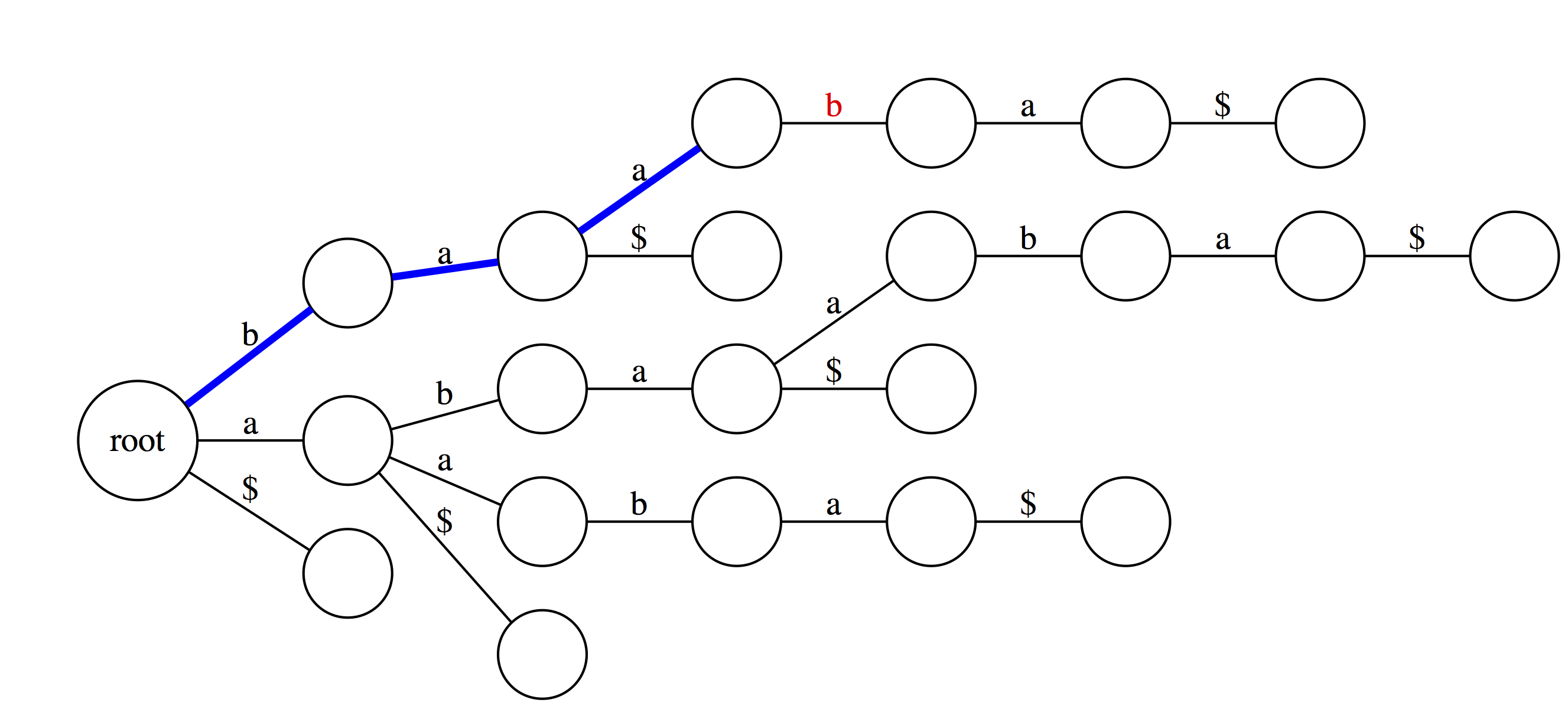
We can also use suffix trie to check if a string is a suffix of a text. You can see that `baa` is **not** a suffix. This is because although it is valid substring, which traces a path through the trie, such path does not with an outgoing edge labeled with `$`.
Here `aba` is a suffix because one of the outgoing edges from the final node is labeled with `$`.</small>
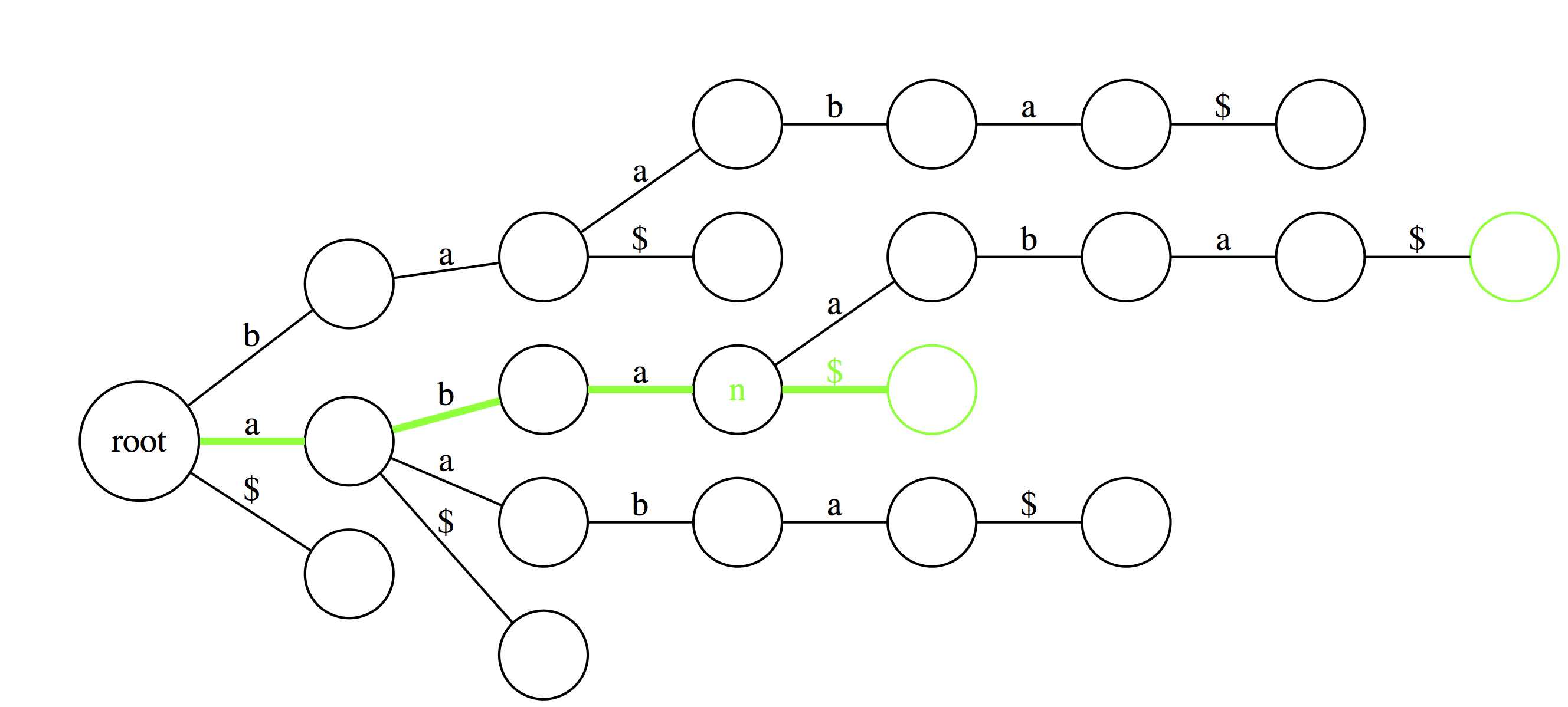
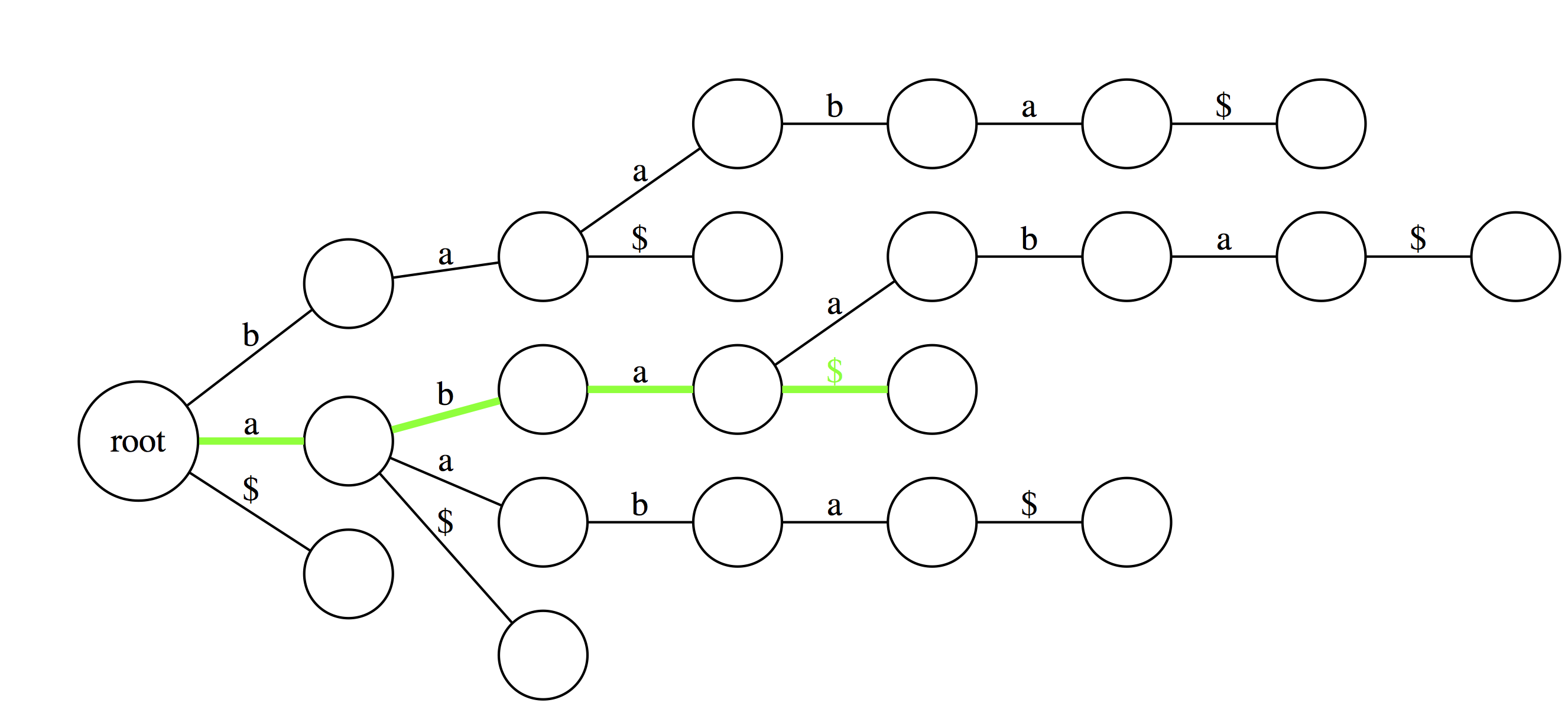
Another useful feature of suffix trie is the ability to tell how many times a particular substring if found in a text. Here `aba` is found twice as the last edge of a path spelling `aba` leads to a node (`n`) with two outgoing edges.
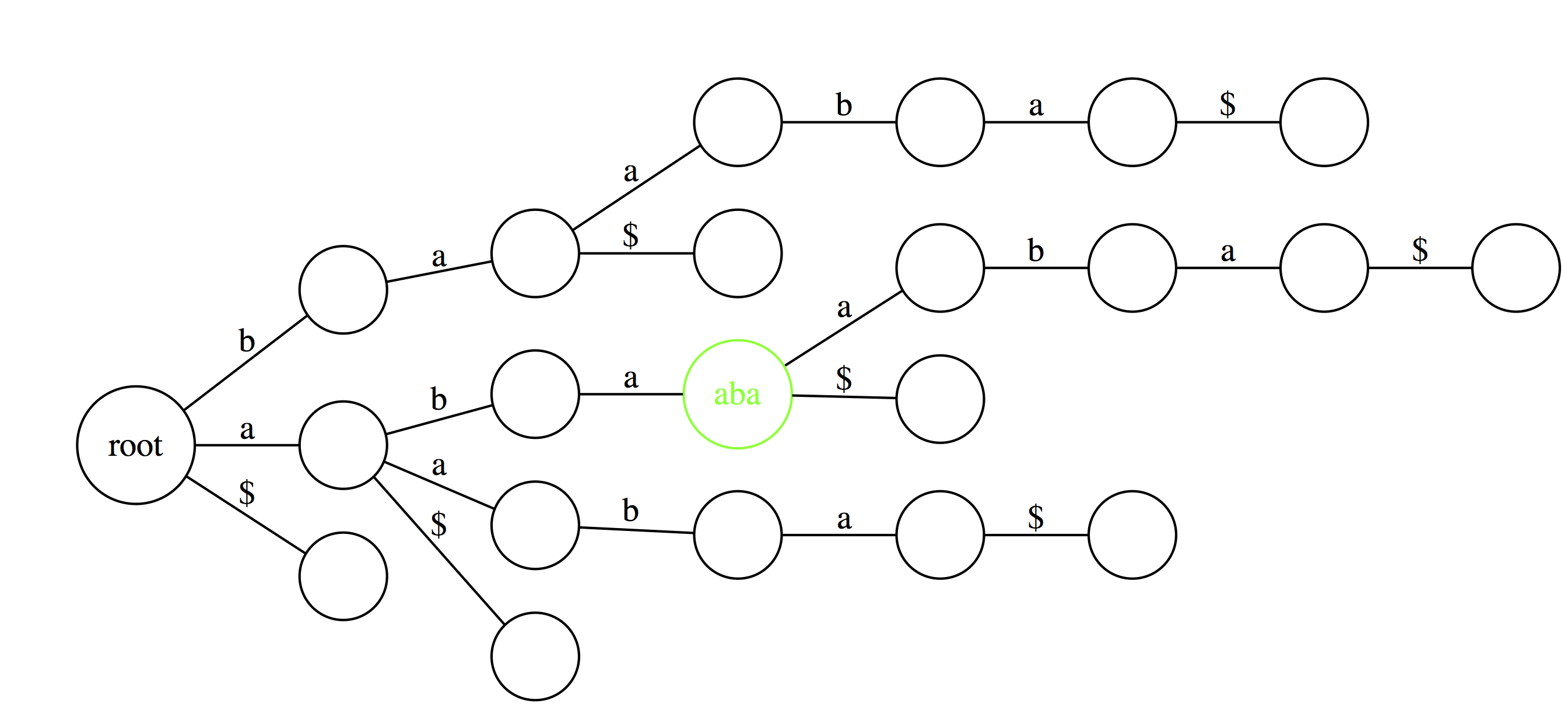
Finally, similar logic allows to find the longest repeated substrings within a text. A deepest (furthest from the root) node with multiple outgoing edges wound point to a repetitive substring. Here `aba` is the longest repeated substring of `abaaba`.
-----
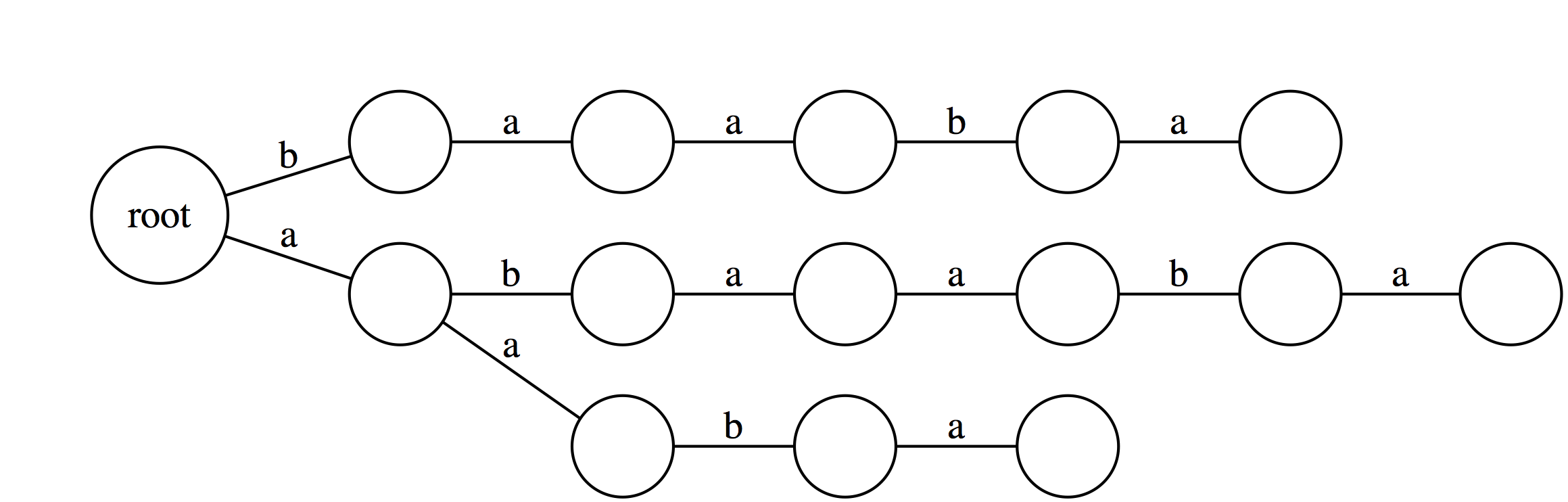
Now that we explained how suffix tries can be used to find substrings in text, let's reduce non-branching paths in tries and convert them to trees:
### From a Trie to a Tree

If we collapse all non-branching paths and concatenate their labels we will get:
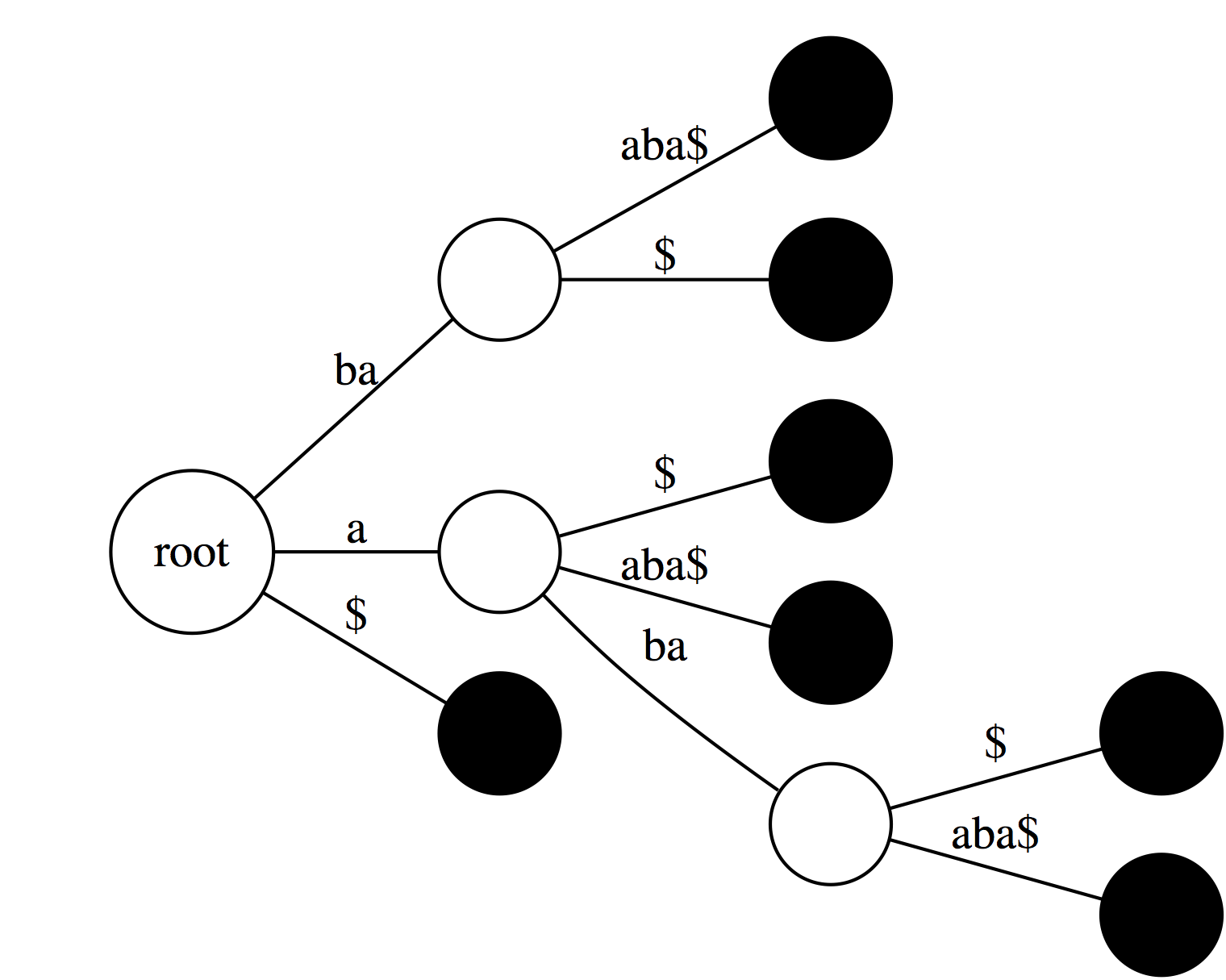
Now, let's label every leaf of the tree with offset (position in the text) of the corresponding suffix:
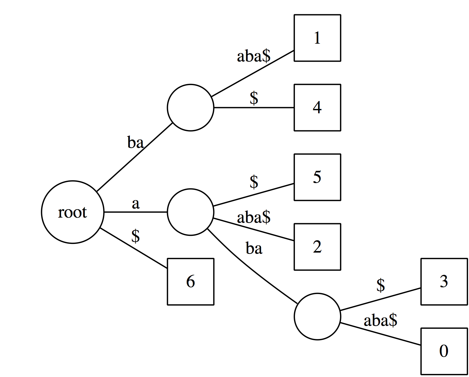
Collapsing non-branching paths has given us a somewhat more compact data structure. Now see how we can use this data structure.
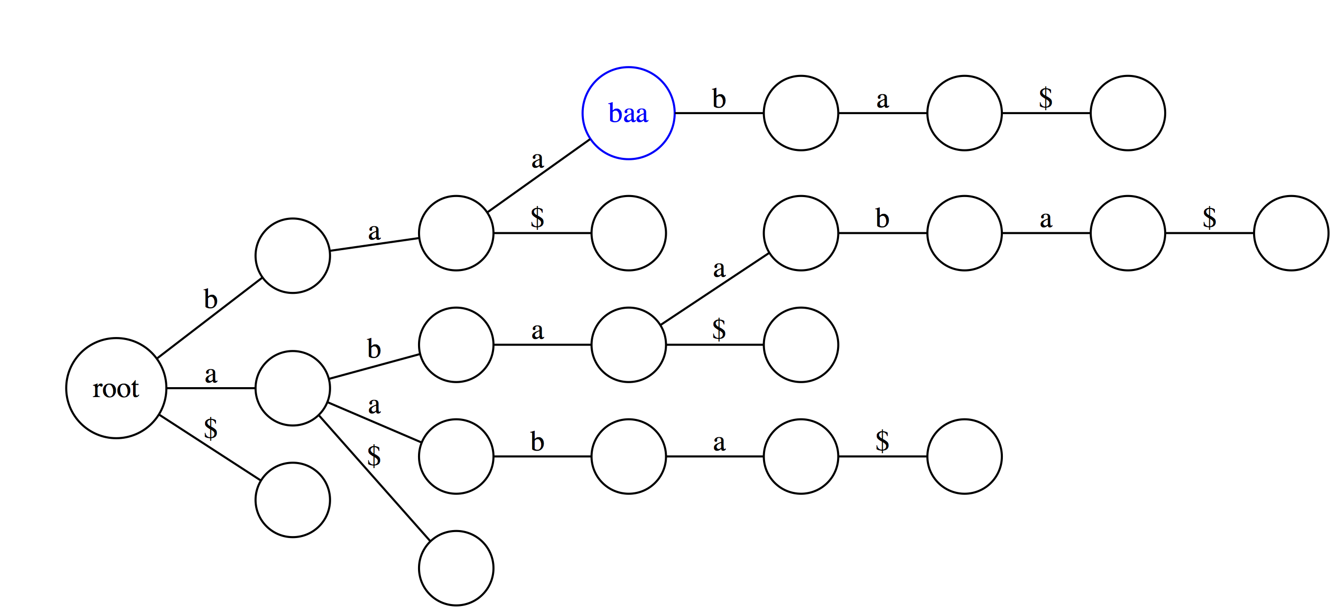
----
### Looking for substrings in a Tree
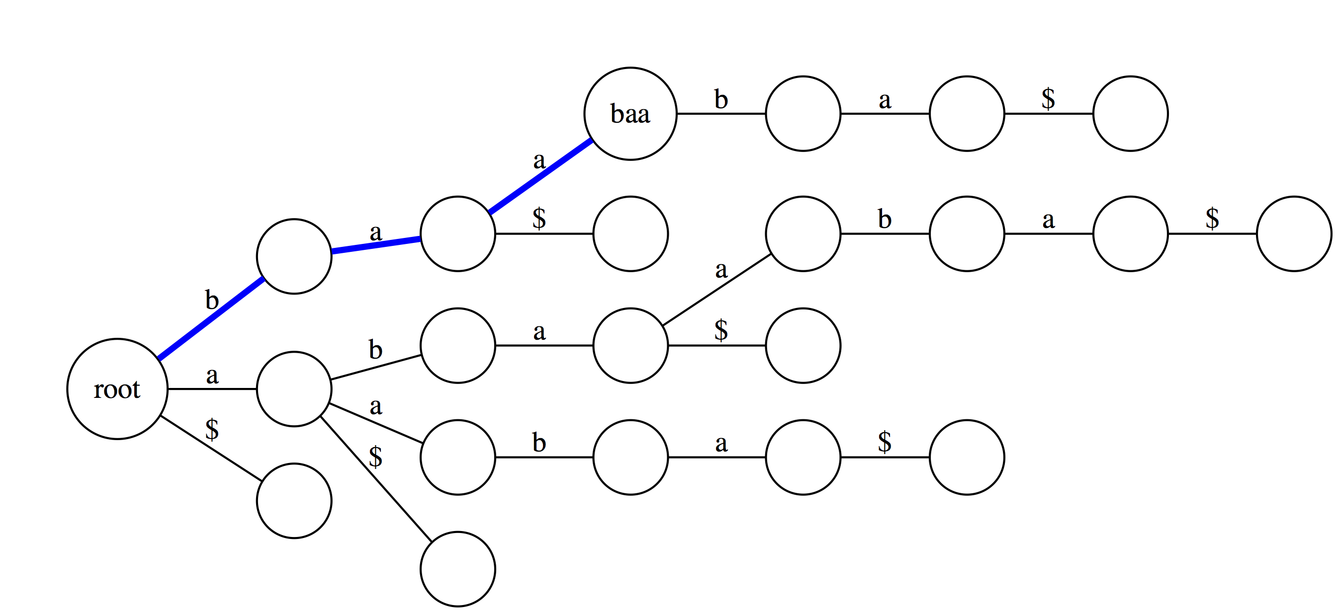
----
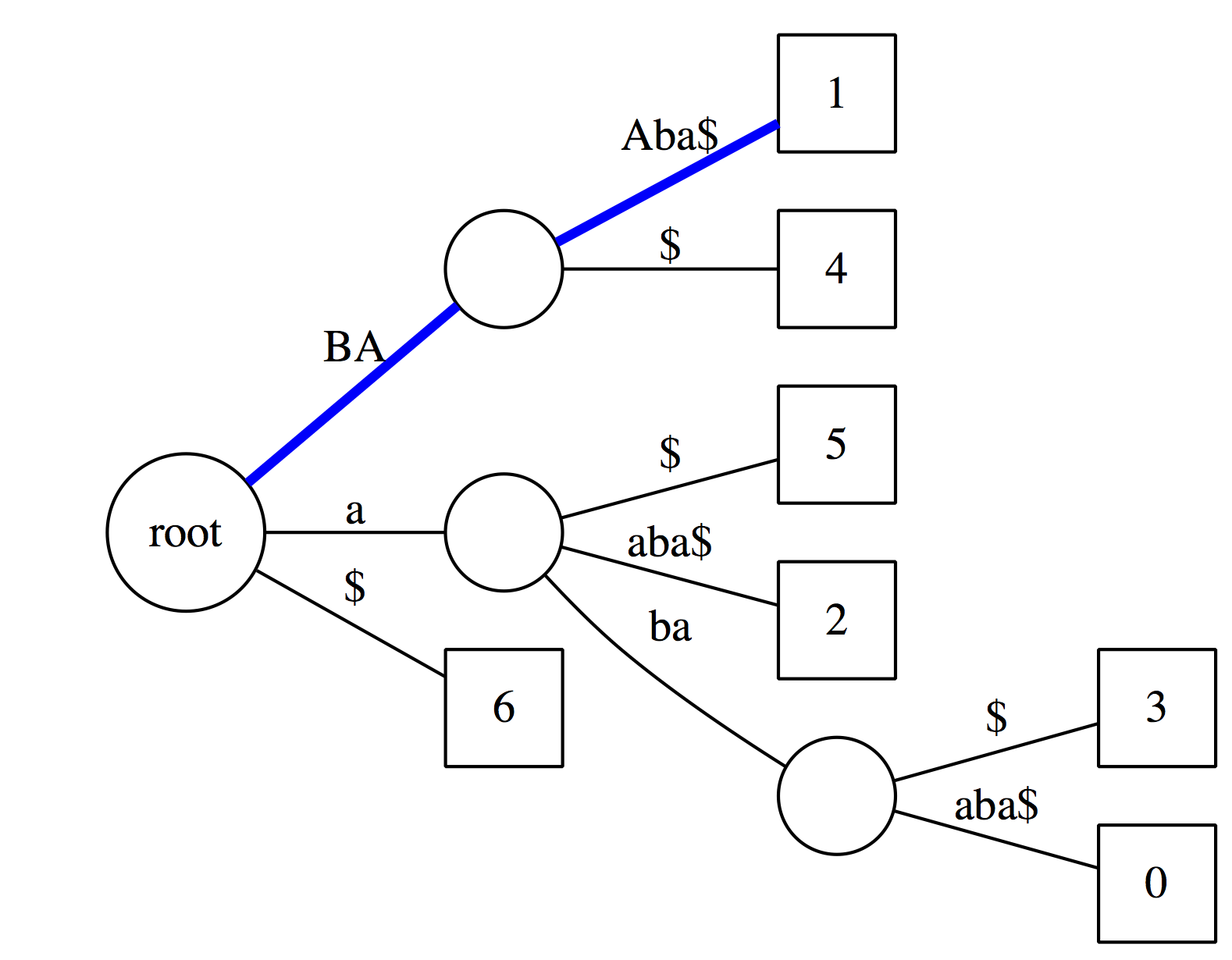
Checking the above suffix tree to see if `baa` is a substring of the text. The logic is exactly the same as with suffix tries, except we now have to account for the fact that along some edges only a portion of the characters within a label will match. In this case matching characters are highlighted with uppercase: `BA` matches along the first edge along the blue path, and only `A` matches along the second edge. The conclusion is that `baa` is a substring of the text.
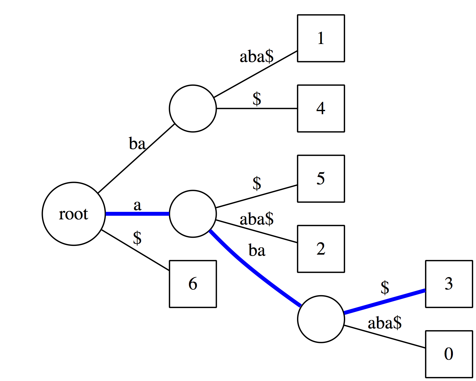
Now let's see if `aba` is a suffix of our text. It matches along the blue path and the last node along this path has an outgoing edge labeled with `$`. Thus it is a suffix.
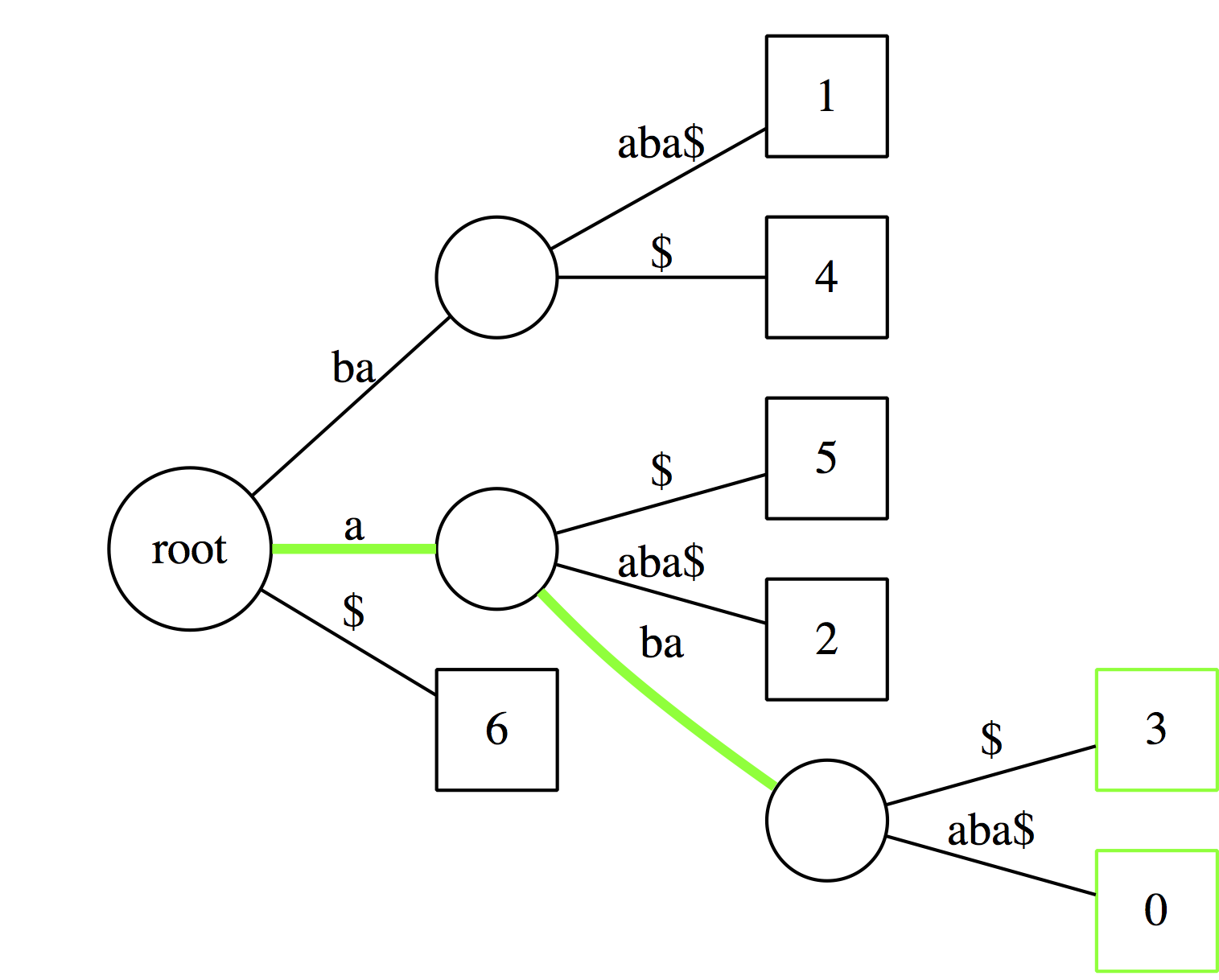
And just like with suffix tries we can count occurrences of a substring by counting the number of outgoing edges from the last node.
------
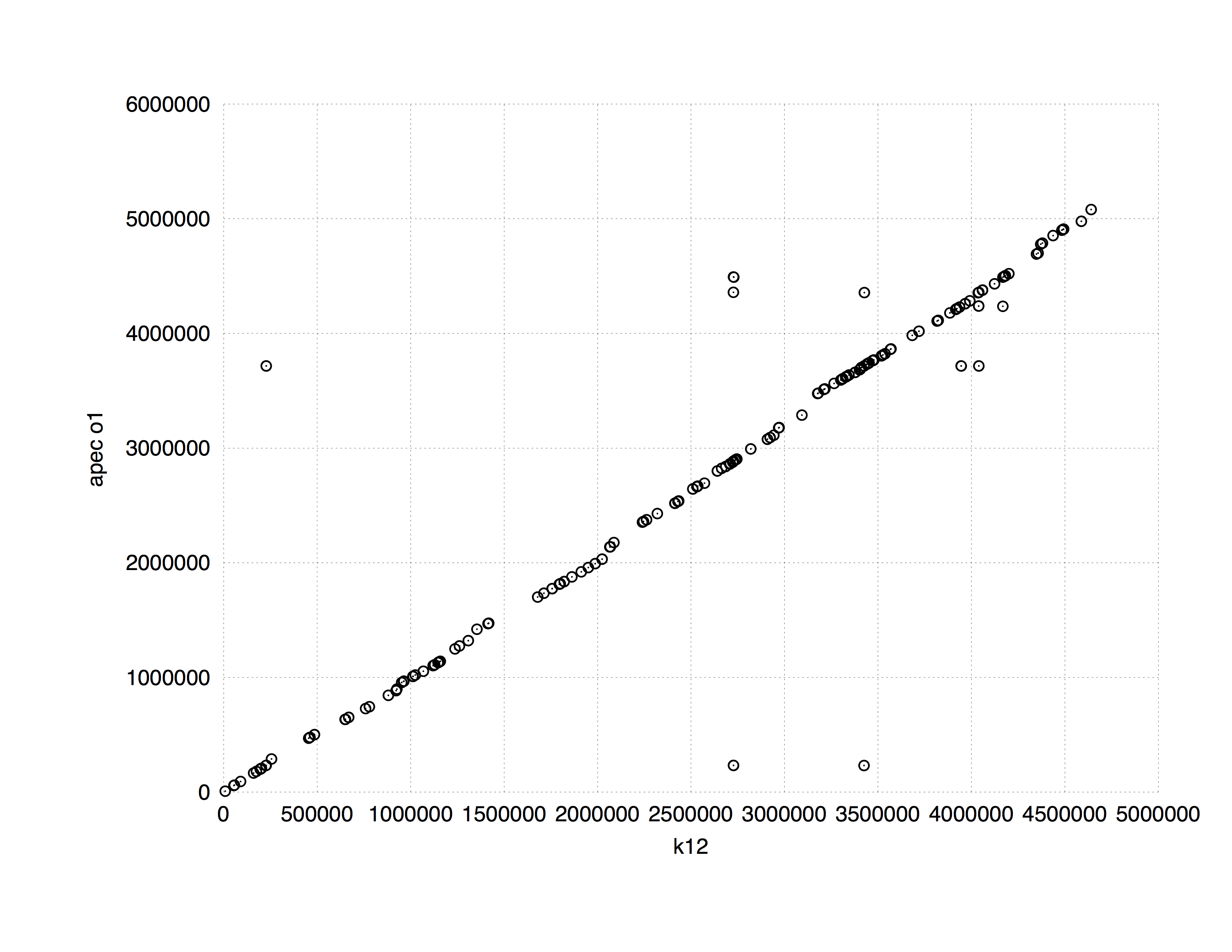
### Application of suffix trees
One of the common applications of suffix trees to the genome data analysis is finding (longest) common subsequences between two sequences. [MUMMER](http://mummer.sourceforge.net/manual/) implements this approach. The following plot shows a comparison between *E. coli* K12 and APEC O1 strains. It is computed in 8 seconds using approximately 10 Mb of RAM (K12 and APEC O1 genomes are 4.5 and 4.9. Mb, respectively).
-----
To find longest common subsequences a suffix tree can be constructed from both sequences at once as shown in the following slide from [Ben Langmead](http://www.cs.jhu.edu/~langmea/resources/lecture_notes/suffix_trees.pdf):
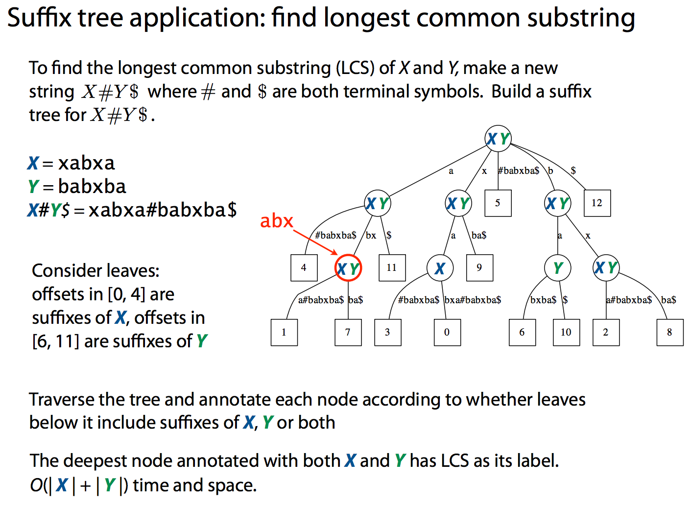
While suffix trees allow sequence comparisons to be performed in nearly linear time, they have large memory footprint. At some point this becomes a serious limitation making the use of suffix trees impractical. For example, indexing human genome will require ~47 Gb of memory.
-----
### Suffix arrays
Suffix array offers a more compact solution to representing text suffixes. It specified a lexicographic ordering of suffixes derived from text *T*$:
---
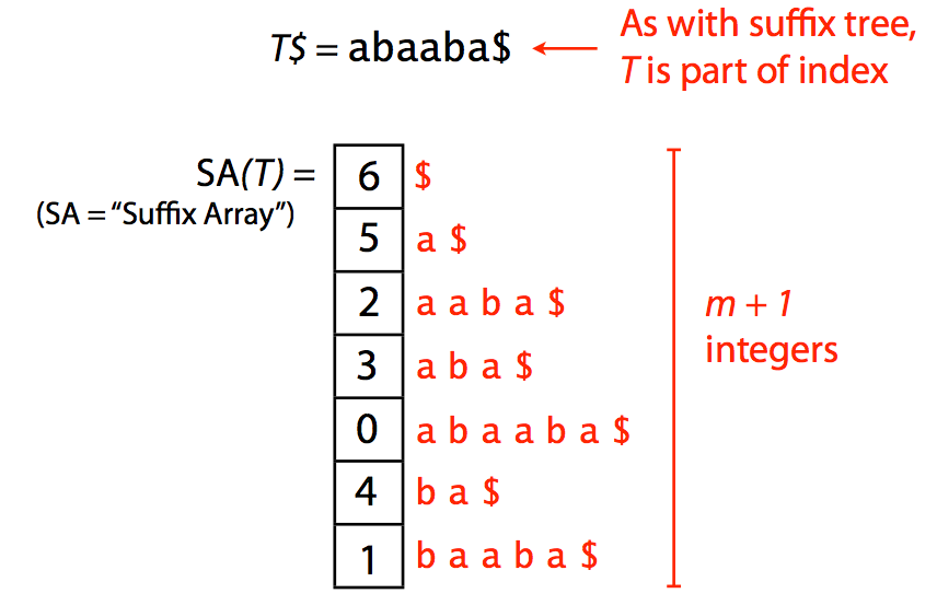
A suffix array. Image by [Ben Langmead](http://www.cs.jhu.edu/~langmea/resources/lecture_notes/indexing_with_substrings.pdf)
----
Because one does not need additional pointers required for tree representation, the suffix array (SA) has a significantly smaller memory footprint. For example, SA for human genome will occupy ~12Gb (down from 47Gb required for a suffix tree). Yet there is an even better idea.
## Burrows-Wheeler Transform and FM index
Burrows-Wheeler (BW) transform is a reversible permutation of a string. For example, for a string:
```
abaaba$
```
create all rotations:
```
$abaaba
a$abaab
ba$abaa
aba$aba
aaba$ab
baaba$a
abaaba$
```
sort them lexicographically with `$` as first character:
```
$abaaba
a$abaab
aaba$ab
aba$aba
abaaba$
ba$abaa
baaba$a
```
take the last column. It will be the BWT of the original string `abaaba$`:
```
abba$aa
```
:::info
Simple python representation is [here](https://colab.research.google.com/github/BenLangmead/comp-genomics-class/blob/master/notebooks/CG_BWT_SimpleBuild.ipynb).
:::
Below is the entire procedure as one slide:
----
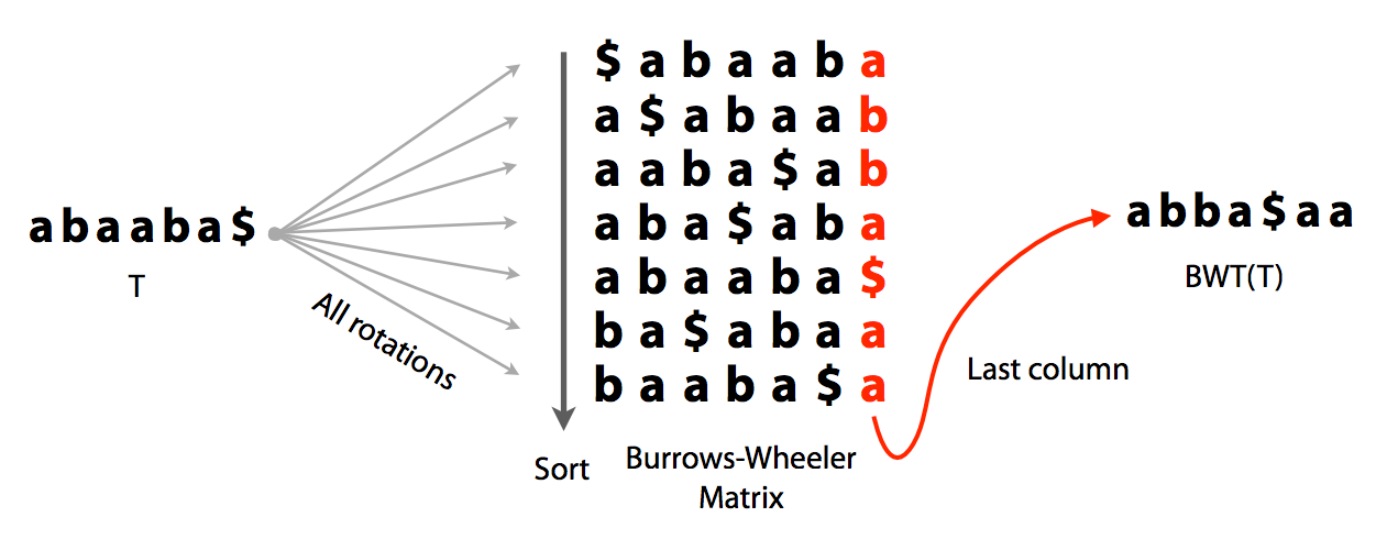
Burrows-Wheeler transform. Image by [Ben Langmead](http://www.cs.jhu.edu/~langmea/resources/lecture_notes/indexing_with_substrings.pdf).
----
It has three important features that make it ideal for creating searchable compact representations of genomic data:
* It can be compressed
* It can be reversed to reconstruct the original string
* It can be used as an index
### LF mapping of Burrows-Wheeler Matrix (BWM)
Let's take the original string `abaaba` add `$` and list charters ranks:
**a**<sub>0</sub>**b**<sub>0</sub>**a**<sub>1</sub>**a**<sub>2</sub>**b**<sub>1</sub>**a**<sub>3</sub>$
This ranking is done based on the order of the characters in the text (T-ranking). The order of ranked characters is preserved between the first column (F) and the last column (L):
----
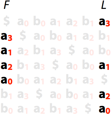
LF mapping: **a**<sub>s</sub> has the same order in F and L
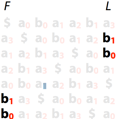
LF mapping: **b**<sub>s</sub> has the same order in F and L. Image by [Ben Langmead](http://www.cs.jhu.edu/~langmea/resources/lecture_notes/indexing_with_substrings.pdf)
----
Let's now rank characters in order of their appearance in the sorted list of rotations (B-ranking):
-----
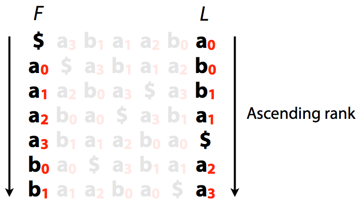
Burrows-Wheeler transform with B-rankings. Image by [Ben Langmead](http://www.cs.jhu.edu/~langmea/resources/lecture_notes/indexing_with_substrings.pdf)
----
A very important implication of this is that we can quickly jump from L to F:
-----
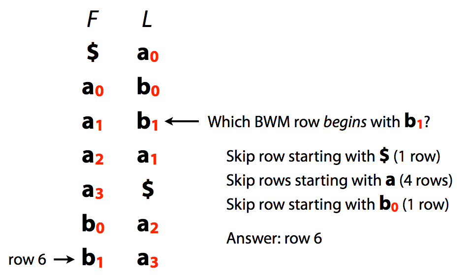
L/F mapping. Image by [Ben Langmead](http://www.cs.jhu.edu/~langmea/resources/lecture_notes/indexing_with_substrings.pdf)
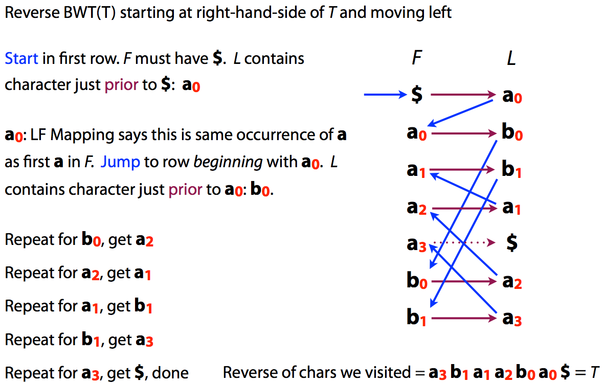
### Reversing BTW
Because of the LF mapping property was can also easily reconstruct original text from its BWT:
----
or
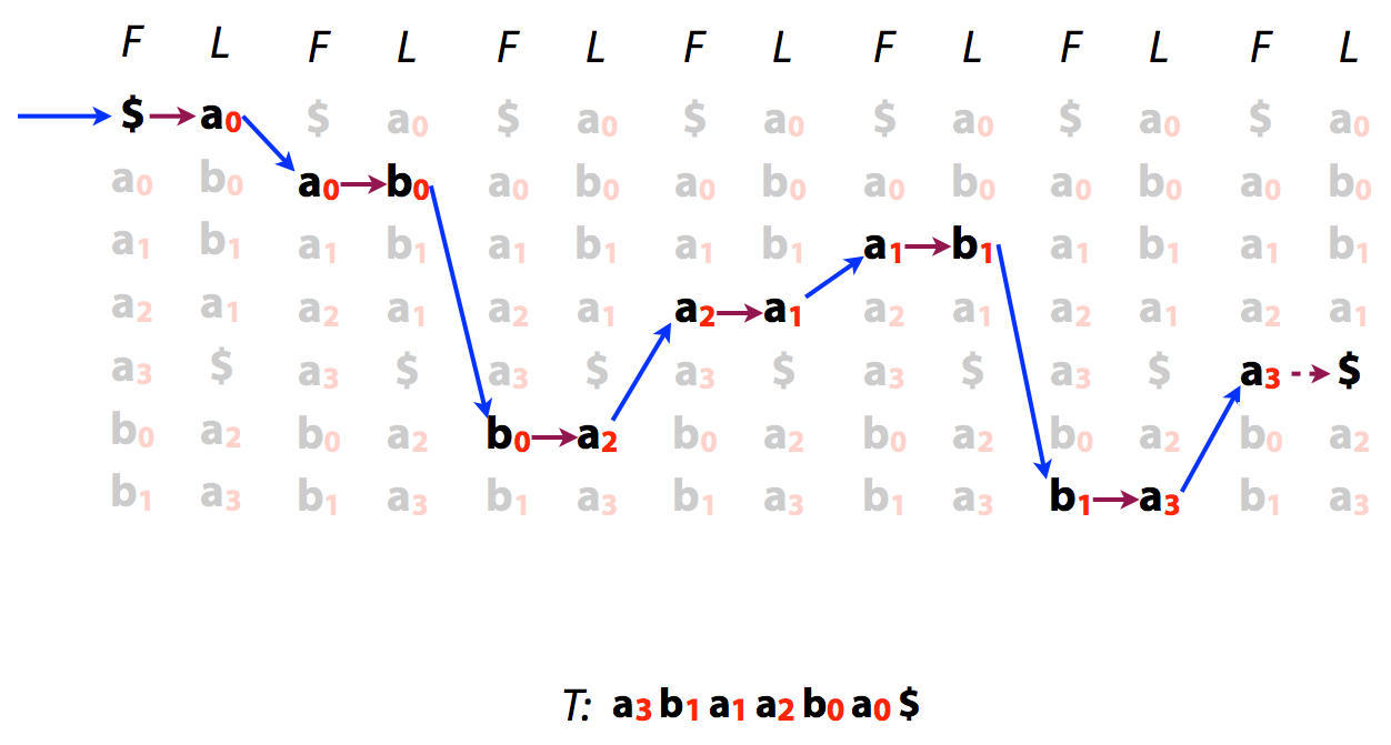
Reversing BWT. Image by [Ben Langmead](http://www.cs.jhu.edu/~langmea/resources/lecture_notes/indexing_with_substrings.pdf)
----
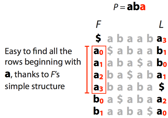
### Searching BWT
Let's try to find is the string `aba` is present in a "genome" stored as a BWT.
---
We start with suffix of $ab\color{red}a$ shown in red. This gives us a range of characters in the F column (all **a**s)
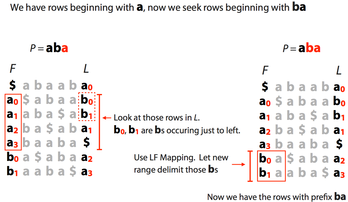
We now extend to $a\color{red}{ba}$ and see how many of **a**s have preceding **b**s:
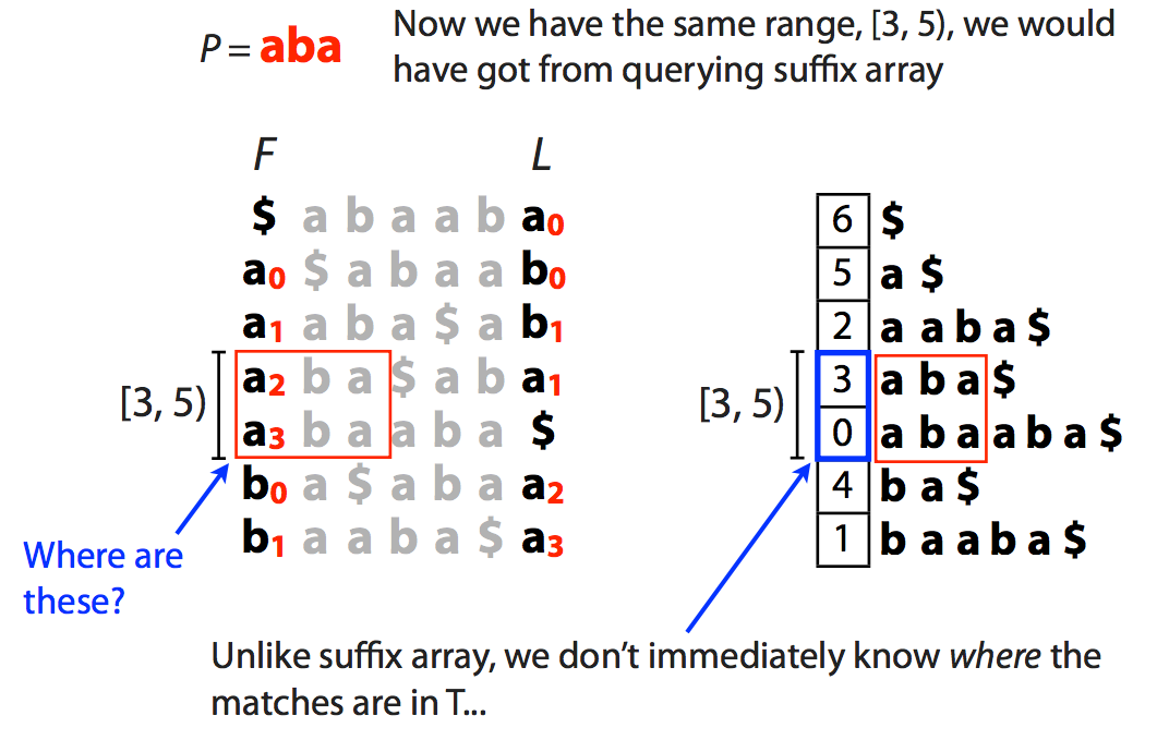
Finally we extend to the entire string $\color{red}{aba}$:
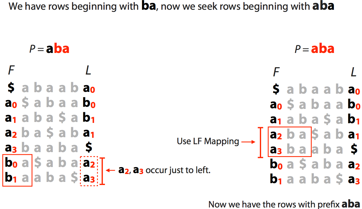
This tells us the range [3,5) but, as opposed to suffix array, this does not tell us where these matches occur in the actual sequence. We will come back to this problem shortly.
The slide below shows what happens when a match is **not** present in the "genome":
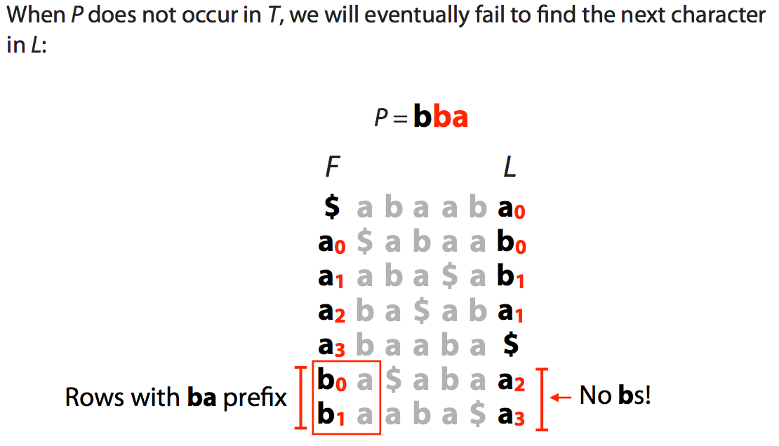
Querying BWT. Images from [Ben Langmead](http://www.cs.jhu.edu/~langmea/resources/lecture_notes/bwt_and_fm_index.pdf)
### Practicalities of using BWT
As we have seen BWT is **very** compact but has few shortcomings such as, for example, the difficulty is seeing where the matches are in the actual genome as well as some performance limitations. Combining BWT with auxiliary data structures creates [FM-index](https://en.wikipedia.org/wiki/FM-index) (where FM stands for Full-text index in Minute space; curiously, the names of FM-index creators are [Ferrigina and Manzini](http://dl.acm.org/citation.cfm?id=796543)). The components of FM-index used for aligning reads to a genome are:
```
BWT Tally Check
points
SA
F L a b a b SA sample
--------- ----- ----- ---- --------
$ abaab a 1 0 1 0 6 $ 6
a $abaa b 1 1 5 a$
a aba$a b 1 2 2 aaba$ 2
a ba$ab a 2 2 2 2 3 aba$
a baaba $ 2 2 0 abaaba$ 0
> b a$aba a 3 2 4 ba$ 4
b aaba$ a 4 2 4 2 1 baaba$
```
Where:
#### BWT
BWT - the BWT (L column from above) is stored and the first column (F) can be easily reconstructed as it is simply a list of all characters (4 in the case of DNA) and their counts.
#### Tally
Because we do not explicitly store ranks they can simply be obtained by counting occurrences of individual characters from the top of L column. Yet this is computationally expensive. Instead we store a tally table. At every row of the BWT matrix it shows how many times each character has been seen up to this point. For example at row marked with `>` there were 3 As and 2 Bs up to this point. In reality, to save space, only a subset of Tally entries is stored as *Checkpoints* recorded in regular intervals as shown above.
#### SA Sample
Finally, to find coordinates of matches in the genome offsets from an SA index are stored as SA sample (actual suffixes are not stored). This allows quickly finding location of a match within the genome by a direct look up. Similarly to Checkpoints only a fraction of these is stored to save space.
Thus the final list of components is:
* First column = integers corresponding to character type counts. In case of DNA four integers: number of As, Cs, Gs, and Ts.
* Last column = the BWT transform. Size is equal to the length of the original text
* Checkpoints = length of text $\times$ number of character types $\times$ sampling fraction (how sparse rows are sampled)
* SA sample = length of text $\times$ fraction of the rows kept
For human genome with DNA alphabet of four nucleotides, saving checkpoint every 128<sup>th</sup> row, and saving SA offsets every 32<sup>nd</sup> row we will have:
* First column = 16 bytes
* Last column = 2bit $\times$ 3 billion characters = 750 MB
* Checkpoints = 3 billion $\times$ 4 bytes/char ÷ 128 ≈ 100 MB
* SA sample = 3 billion $\times$ 4 bytes/char ÷ 32 ≈ 400 MB
 Sign in with Wallet


