W4 - Dispersion, Principal Component Analysis
===

## 名字: 鄭詩蓉
### KMO 取樣適切性量數（Kaiser-Meyer-Olkin Measure of Sampling Adequacy）

- KMO 是做**主成分分析（PCA）或因素分析之前**，用來確認「這批資料到底適不適合進行降維分析」的前提檢驗指標。
- 如果變數之間的相關是「由某個共同的潛在因素所驅動的」，那就值得做 PCA；如果相關只是各自偶然、表面上的，硬做 PCA 沒有意義。
- 數值範圍：**0 到 1**，越接近 1 代表資料越適合；**低於 0.5 不應進行 PCA**。

---

#### 需要先懂的兩個概念

- **相關係數（Correlation Coefficient）$r_{ij}$**：直接觀察到的「兩個變數之間的相關程度」。
- 例如：數學成績和理化成績之間的相關係數是 0.8。
- 這個相關可能是因為背後有「理科能力」這個共同因素在驅動，也可能只是剛好。

- **淨相關係數（Partial Correlation）$p_{ij}$**：在**控制其他所有變數的影響之後**，兩個變數之間「純粹剩下的相關」。
- 例如：控制掉「整體努力程度」這個共同因素後，數學和理化還剩下多少相關？
- 如果控制後相關大幅縮小，代表原本的相關確實是被共同因素帶動的（好事！KMO 會高）。
- 如果控制後相關依然很高，代表這兩個變數的相關並不依賴共同因素（KMO 會低）。

> **例子**：
> 假設你發現「吃冰淇淋的量」和「溺水人數」高度相關（$r = 0.9$）。
> 但一旦你控制掉「夏天（氣溫）」這個共同因素，兩者就幾乎不相關了（$p \approx 0$）。
> 這說明原本的相關完全是被「夏天」這個潛在因素造成的，而這正是 PCA 想挖掘的結構。

---

#### 公式

$$KMO = \frac{\displaystyle\sum_{i \neq j} r_{ij}^2}{\displaystyle\sum_{i \neq j} r_{ij}^2 + \displaystyle\sum_{i \neq j} p_{ij}^2}$$

- $r_{ij}$：變數 $i$ 和 $j$ 的**觀察相關係數**（直接測量到的相關）
- $p_{ij}$：變數 $i$ 和 $j$ 的**淨相關係數**（控制其他變數後的殘餘相關）
- $\sum_{i \neq j}$：對所有不同的變數對求加總（不包含自己跟自己）

**公式解讀：**

$$KMO = \frac{\text{真實的共同因素造成的相關}}{\text{真實的共同因素造成的相關} + \text{控制後還剩下的偶然相關}}$$

→ 淨相關（$p$）越小，分母越小，KMO 越大 → 資料越適合做 PCA
→ 淨相關（$p$）越大，分母越大，KMO 越小 → 資料不適合做 PCA

---

#### 例子：學生成績裡有沒有「共同因素」？

> **情境**：某老師想知道學生的「國文」、「英文」、「數學」三科成績背後，是否有可以被 PCA 抓出來的共同結構。她先做 KMO 檢驗。

**Step 1：列出觀察相關係數 $r$（兩兩之間直接的相關）**

| 變數對 | 觀察相關係數 $r$ | $r^2$ |
|--------|----------------|--------|
| 國文 ↔ 英文 | 0.80 | 0.6400 |
| 國文 ↔ 數學 | 0.70 | 0.4900 |
| 英文 ↔ 數學 | 0.75 | 0.5625 |
| **合計** | | **1.6925** |

**Step 2：列出淨相關係數 $p$（控制第三科後，剩餘的相關）**

> 淨相關通常比觀察相關小很多。這裡直接套假設好的數字，實際上由統計軟體算出。

| 變數對 | 淨相關係數 $p$ | $p^2$ |
|--------|--------------|--------|
| 國文 ↔ 英文（排除數學影響） | 0.20 | 0.0400 |
| 國文 ↔ 數學（排除英文影響） | 0.15 | 0.0225 |
| 英文 ↔ 數學（排除國文影響） | 0.10 | 0.0100 |
| **合計** | | **0.0725** |

**Step 3：代入公式**

$$KMO = \frac{1.6925}{1.6925 + 0.0725} = \frac{1.6925}{1.765} \approx \mathbf{0.959}$$

**結論：KMO = 0.959，屬於「極佳」等級，這筆成績資料非常適合進行 PCA！**

> 為什麼這麼高？因為淨相關（0.0725）比觀察相關（1.6925）小非常多，代表三科之間的相關幾乎都是被「某個共同因素（例如整體學業能力）」所驅動的，控制後幾乎沒有剩餘的偶然相關。

---

#### 搭檔：Bartlett's Test of Sphericity（巴特利球形檢定）

KMO 幾乎一定要搭配 **Bartlett's Test** 一起報告。

**Bartlett 在問什麼？**
「這些變數的相關矩陣，是否顯著地**不是一個單位矩陣（Identity Matrix）**？」

**單位矩陣是什麼？**（以三個變數為例）

| | 國文 | 英文 | 數學 |
|--|------|------|------|
| 國文 | **1** | 0 | 0 |
| 英文 | 0 | **1** | 0 |
| 數學 | 0 | 0 | **1** |

> 對角線都是 1（自己跟自己的相關永遠是 1），其他格子全是 0，代表所有變數彼此**完全獨立、沒有任何相關**。
> Bartlett 就是在問：「你的資料矩陣，是不是跟這個『各自獨立』的矩陣顯著不同？」如果顯著不同，才代表變數之間真的有相關，PCA 才有意義。

**判斷結果：**
- 資料和單位矩陣**顯著不同（p < .05）** → 變數之間有相關 → 可以做 PCA
- 資料和單位矩陣**沒有顯著不同（p ≥ .05）** → 大家各自獨立 → 不適合做 PCA

**Bartlett 的自由度（df）怎麼算？**

$$df = \frac{k(k-1)}{2}$$

- $k$：你有幾個變數
- 邏輯：$k$ 個變數兩兩配對，總共有幾種不重複的組合，就是幾個自由度

> 以本論文為例，共有 **8 個詞彙指標變數**：
>
> $$df = \frac{8 \times (8-1)}{2} = \frac{8 \times 7}{2} = \frac{56}{2} = 28$$
>
> 所以reading寫的 $\chi^2(28)$，括號裡的 28 就是這樣算出來的

**Bartlett 的缺點——對樣本數非常敏感：**
只要樣本數夠大（例如超過 1,000 筆），Bartlett 幾乎一定會顯著，即使相關很低。
因此 Bartlett 顯著只能當「參考」，**最重要的判斷依據還是 KMO**。

---

#### SPSS 示意圖


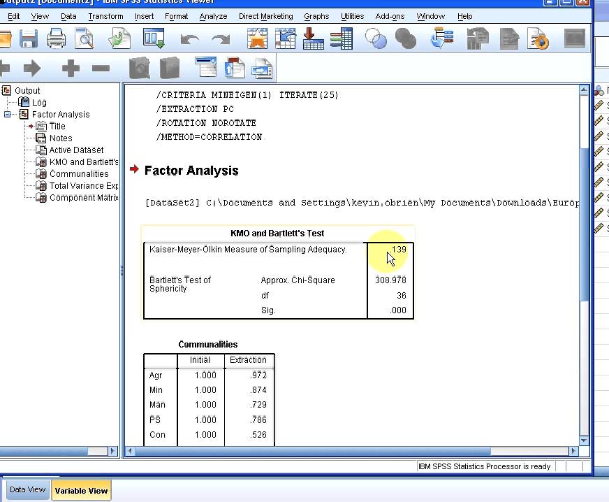
> SPSS 輸出的「KMO 與 Bartlett 的球形檢定」表格，上方是 KMO 值，下方是 Bartlett 的 χ² 值與顯著性（Sig.）。只要 KMO ≥ 0.6 且 Sig. < .05，就可以繼續進行 PCA。

---

#### 對應 Reading 裡的數字

分析了 **7,799 個英語單字**的 **8 個詞彙指標**，在進行 PCA 之前先做了 KMO 檢驗：

- **KMO = .715**（中等，通過 ≥ 0.6 的門檻）
- **Bartlett's Test：$\chi^2(28) = 1439.98,\ p < .001$**（顯著，通過）
- df = 28，正是因為有 8 個變數：$\frac{8 \times 7}{2} = 28$

因此兩項前提檢驗均通過，可以正式進入主成分分析（PCA）。

---

#### KMO 數值解讀標準

| KMO 值 | 解讀 |
|--------|------|
| 0.90 以上 | 極佳（Marvelous） |
| 0.80 ~ 0.89 | 良好（Meritorious） |
| 0.70 ~ 0.79 | 中等（Middling） |
| 0.60 ~ 0.69 | 平庸（Mediocre） |
| 0.50 ~ 0.59 | 不太適合（Miserable） |
| **0.50 以下** | **不可接受，不應做 PCA** |

---

#### 複習

> **KMO 原則**：
> 「分子是觀察相關的平方和，分母是分子再加上淨相關的平方和」
> 淨相關越小 → 分母越小 → KMO 越大 → 資料越好

> **Bartlett df 原則**：
> $df = \dfrac{k(k-1)}{2}$，$k$ 個變數兩兩配對的總組合數

> **下一步**：KMO 與 Bartlett 都通過後，就可以進入**主成分分析（PCA）**。

---

#### 資料來源

- 點部落 tingi. (2019). *[R] 讀取 sav 檔產生 SPSS 的 KMO 及 Bartlett 球形檢定*. [https://dotblogs.com.tw/tingi/2019/09/16/135950](https://dotblogs.com.tw/tingi/2019/09/16/135950)
- 文化大學數位學習中心. (n.d.). *SPSS 進階分析：因素分析*. [http://digilc.sce.pccu.edu.tw/download/SPSS%E9%80%B2%E9%9A%8E%E5%88%86%E6%9E%90_%E6%8E%A8%E5%BB%A3%E9%83%A8.pdf](http://digilc.sce.pccu.edu.tw/download/SPSS%E9%80%B2%E9%9A%8E%E5%88%86%E6%9E%90_%E6%8E%A8%E5%BB%A3%E9%83%A8.pdf)
- 國立高雄科技大學. (n.d.). *因素分析（Factor Analysis）*. [http://www2.nkust.edu.tw/~tsungo/Publish/26%20Factor%20Analysis.pdf](http://www2.nkust.edu.tw/~tsungo/Publish/26%20Factor%20Analysis.pdf)
- 國立體育大學. (n.d.). *因素分析大綱*. [http://www.epsport.net/sportscience/database/factor.pdf](http://www.epsport.net/sportscience/database/factor.pdf)
- Zhang, H., Han, Y., Zhang, X., & Cui, L. (2022). Frequency, Dispersion and Abstractness in the Lexical Sophistication Analysis of A Learner-Based Word Bank. *Journal of Quantitative Linguistics*, 29(2), 195–211. [https://doi.org/10.1080/09296174.2020.1782716](https://doi.org/10.1080/09296174.2020.1782716)
---
### 主成分分析（PCA, Principal Component Analysis）

- PCA 是一種**降維技術（Dimensionality Reduction）**，把「很多個互相相關的變數」壓縮成「少數幾個有代表性的主成分」，同時盡量保留最多資訊量。
- 使用時機：懷疑手上的很多變數背後，其實只有幾個核心概念在主導，想把這些核心「挖出來」並為它們命名。

> **打個比方**：
> 想了解一個學生的學習狀況，你有「每週補習時數、作業完成率、課堂發問次數、自習時間、練習題完成量」5 項資料。
> 這 5 項其實背後都在反映同一件事：**這個學生有多努力**。
> PCA 就是把這 5 項資料壓縮成 1 個「努力程度指數」。

---

#### 五個重要的基本概念

- **變異量（Variance）**：一組數字的分散程度。越分散，代表這個變數越有「區別力」（能看出誰高誰低）。PCA 就是找「保留最多區別力的方向」。

- **主成分（Principal Component, PC）**：PCA 計算出來的新變數，是原始變數的加權總和。PC1 保留最多變異，PC2 保留第二多，且每個主成分彼此**完全不重疊**。

- **特徵值（Eigenvalue）**：每個主成分解釋了多少變異量。原本有幾個變數，特徵值加總就等於幾。例如 8 個變數，8 個特徵值加起來 = 8。

- **因子負荷量（Factor Loading）**：每個原始變數跟每個主成分之間的相關係數，告訴你「這個變數最屬於哪個主成分」。越接近 1（或 -1），歸屬越強。

- **共同度（Communality）**：一個原始變數「有多少比例的資訊被 PCA 保留下來」。越高越好，一般要求 >= 0.5。

---

#### PCA 完整流程（五個步驟）

【有很多個相關變數】
        ↓
Step 1  資料標準化（讓變數站在同一起跑線）
        ↓
Step 2  計算特徵值（決定每個主成分有多重要）
        ↓
Step 3  用特徵值 > 1 + 陡坡圖決定保留幾個主成分
        ↓
Step 4  因子旋轉（讓負荷量更集中，結果更好讀懂）
        ↓
Step 5  讀因子負荷量表，為每個主成分命名

---

#### Step 1：資料標準化（Standardization）

**為什麼要標準化？**

不同變數的單位不同，數字大小差很多，如果直接計算，數字大的變數會霸占結果，不公平。標準化讓每個變數的平均 = 0、標準差 = 1，站在同等起跑線。

**標準化公式：**

$$z = \frac{x - \bar{x}}{s}$$

- $x$：某人的原始數值
- $\bar{x}$：這個變數的平均值
- $s$：這個變數的標準差

#### 例子：補習時數與成績的標準化

某班調查了「每週補習時數」和「考試成績」：

| 學生 | 補習時數 $x$ | 平均 $\bar{x}$ | 標準差 $s$ | 標準化後 $z$ | 計算過程 |
|------|------------|--------------|-----------|------------|---------|
| 小明 | 10 小時 | 6 小時 | 2 小時 | **+2.0** | $(10-6)\div2 = 2.0$ |
| 小花 | 6 小時 | 6 小時 | 2 小時 | **0.0** | $(6-6)\div2 = 0.0$ |
| 小美 | 4 小時 | 6 小時 | 2 小時 | **-1.0** | $(4-6)\div2 = -1.0$ |

> 標準化後的意思：小明補習量比平均高 2 個標準差，小美比平均少 1 個標準差。現在「補習時數」和「考試分數（0~100分）」可以放在同一張分析裡公平比較了。

---

#### Step 2：特徵值（Eigenvalue）——每個主成分有多重要？

**特徵值 = 這個主成分能解釋的變異量**

**解釋變異比例的計算：**

$$\text{解釋變異比例} = \frac{\text{這個主成分的特徵值}}{\text{所有特徵值加總}}$$

#### 例子：護膚研究的特徵值

假設一位美容研究員調查了 5 項護膚指標：
**防曬頻率、保濕乳液使用量、睡眠時間、喝水量、蔬果攝取量**，共 5 個變數，特徵值加總 = 5。

| 主成分 | 特徵值 | 計算解釋比例 | 解釋比例 | 累積比例 | 保留？ |
|--------|--------|------------|--------|---------|-------|
| PC1 | 3.20 | $3.20 \div 5 = 0.640$ | 64.0% | 64.0% | 是（> 1）|
| PC2 | 1.10 | $1.10 \div 5 = 0.220$ | 22.0% | **86.0%** | 是（> 1）|
| PC3 | 0.40 | $0.40 \div 5 = 0.080$ | 8.0% | 94.0% | 否（< 1）|
| PC4 | 0.20 | — | 4.0% | 98.0% | 否（< 1）|
| PC5 | 0.10 | — | 2.0% | 100% | 否（< 1）|

**結論：保留 PC1 + PC2，合計解釋 86% 的總變異。**

---

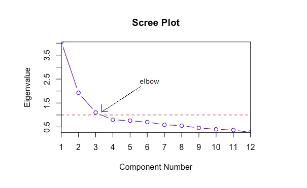
#### Step 3：陡坡圖（Scree Plot）——要保留幾個主成分？

把每個主成分的特徵值由大到小畫成折線圖，找到**曲線開始走平的「手肘點（Elbow Point）」**。手肘點之前的主成分保留，之後的淘汰。


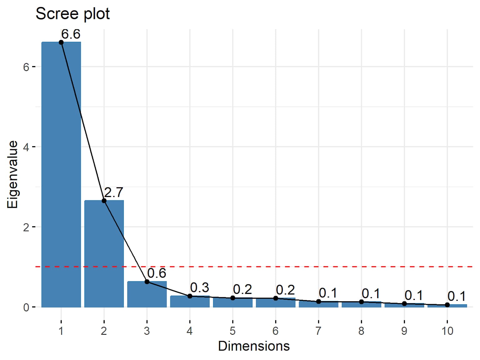
> 圖中可以看到：第 1、2 個主成分的特徵值很高，從第 3 個之後曲線明顯走平（手肘在第 2 個之後）→ 保留前 2 個主成分。

**兩個判斷標準，一起使用才穩：**

| 標準 | 做法 |
|------|------|
| **Kaiser 準則** | 保留**特徵值 > 1** 的主成分 |
| **陡坡圖（Scree Plot）** | 找「曲線彎曲後走平」的手肘點，手肘點之前的全保留 |

---

#### Step 4：因子旋轉（Factor Rotation）

旋轉**不會改變解釋的總變異量**，只是重新分配每個主成分的負荷量，讓每個變數更清楚地「歸屬」到某一個主成分，結果更好讀、更容易命名。

> 旋轉就像調整相機角度——照的是同一個景，但換個角度之後主體更清晰。

| 旋轉方法 | 英文名 | 假設 | 使用時機 |
|----------|--------|------|---------|
| **直交旋轉** | Varimax | 主成分之間**完全獨立，不相關** | 理論上認為因素完全無關時 |
| **斜交旋轉** | Direct Oblimin | 主成分之間**允許有相關** | 現實中因素通常有一定關聯，較貼近真實 |

> **本次reading**使用 **Direct Oblimin（斜交旋轉）**，因為詞彙指標在現實中難以完全獨立。旋轉後兩個主成分的相關係數 $r = .394$，確認有適度相關。

---

#### Step 5：讀因子負荷量表——為主成分命名

因子負荷量 = **每個原始變數與每個主成分之間的相關係數**。

**判斷標準：**

| 負荷量絕對值 | 解讀 |
|-------------|------|
| >= **0.7** | 非常強，這個變數高度屬於這個主成分 |
| >= **0.6** | 強，屬於這個主成分 |
| >= **0.4** | 有意義，可納入考量 |
| < **0.4** | 可忽略，幾乎不屬於這個主成分 |

#### 例子：護膚研究的因子負荷量表

| 變數 | **PC1（外在護膚習慣）** | **PC2（內在養生習慣）** |
|------|----------------------|----------------------|
| 防曬頻率 | **0.91** | 0.05 |
| 保濕乳液使用量 | **0.88** |0.09 |
| 喝水量 | 0.07 | **0.85** |
| 睡眠時間 | 0.10 | **0.82** |
| 蔬果攝取量 | 0.06 | **0.79** |

**怎麼讀這張表？**
1. 找每個變數**負荷量最大**的那一格（粗體格）
2. 同一欄負荷量都高的變數，就「歸屬」到這個主成分
3. 根據這些變數的共同特性，為主成分取一個有意義的名字

→ 防曬頻率、保濕乳液在 PC1 負荷量 > 0.88 → PC1 命名為「**外在護膚習慣**」
→ 喝水量、睡眠、蔬果在 PC2 負荷量 > 0.79 → PC2 命名為「**內在養生習慣**」
→ 結論：影響膚況的 5 個指標，背後只有 2 個核心維度！

#### 護膚研究的共同度

共同度 = 這個變數有多少比例的資訊，被所有保留的主成分「解釋到了」。

$$\text{共同度} = (\text{PC1 負荷量})^2 + (\text{PC2 負荷量})^2$$

> 注意：此公式只適用於**直交旋轉（Varimax）**。若使用斜交旋轉，共同度由軟體直接輸出，不可手算，但解讀邏輯相同。

| 變數 | PC1 負荷量 | PC2 負荷量 | 共同度計算 | 共同度 | 達標（>= 0.5）？ |
|------|-----------|-----------|----------|-------|-----------------|
| 防曬頻率 | 0.91 | 0.05 | $0.91^2 + 0.05^2 = 0.8281 + 0.0025$ | **0.831** | 是 |
| 保濕乳液 | 0.88 | 0.09 | $0.88^2 + 0.09^2 = 0.7744 + 0.0081$ | **0.782** | 是 |
| 喝水量 | 0.07 | 0.85 | $0.07^2 + 0.85^2 = 0.0049 + 0.7225$ | **0.727** | 是 |

> 防曬頻率共同度 = 0.831，代表這個變數有 83.1% 的資訊被 PCA 保留住了，只流失 16.9%。

---

#### 對應 Reading 的結果（Zhang et al., 2022）

本次 Reading 分析 **7,799 個英語單字**的 **8 個詞彙指標**，以下依序呈現 PCA 各項結果。

---

特徵值與解釋變異比例

> 未直接列出特徵值數字，以下依reading（"first component explained 74.5% of the variance and the second component explained 14.7%"）反推：$8 \times 0.745 = 5.96$；$8 \times 0.147 = 1.176$

| 主成分 | 特徵值（反推） | 計算解釋比例 | 解釋比例 | 累積比例 | 保留？ |
|--------|-------------|------------|--------|---------|-------|
| PC1 | 5.96 | $5.96 \div 8 = 0.745$ | **74.5%** | 74.5% | 是（> 1）|
| PC2 | **1.176** | $1.176 \div 8 = 0.147$ | **14.7%** | **89.3%** | 是（> 1）|
| PC3～PC8 | 各 < 1 | — | 10.7% | 100% | 否 |

**結論：保留 PC1 + PC2，合計解釋 89.3% 的總變異。**

---

共同度

| 變數 | 初始值 | 萃取值（共同度） | 達標（>= 0.5）？ |
|------|--------|--------------|----------------|
| COCA 詞頻 | 1.000 | **0.992** | 是 |
| BNC 詞頻 | 1.000 | **0.994** | 是 |
| COCA 口語詞頻 | 1.000 | **0.957** | 是 |
| COCA 學術詞頻 | 1.000 | **0.945** | 是 |
| BNC 口語詞頻 | 1.000 | **0.856** | 是 |
| BNC 學術詞頻 | 1.000 | **0.941** | 是 |
| COCA 分散度 | 1.000 | **0.728** | 是 |
| BNC 分散度 | 1.000 | **0.729** | 是 |

> 所有 8 個變數的共同度均 > 0.7，代表 PCA 對每個原始變數的解釋力都很高，壓縮過程中資訊損失極少。

---

因子負荷量（Direct Oblimin 旋轉後）

> 將抽象性（Abstractness）操作化為「學術語料庫中的詞頻」，因為學術詞彙往往越抽象。因此 COCA 學術詞頻與 BNC 學術詞頻同時代理「詞頻」與「抽象性」兩個概念，這也是為什麼 PC1 被命名為「詞頻 + 抽象性」。

| 變數 | **PC1（詞頻 + 抽象性）** | **PC2（分散度）** |
|------|----------------------|----------------|
| COCA 詞頻 | **0.994** | 0.004 |
| BNC 詞頻 | **0.999** | -0.007 |
| COCA 口語詞頻 | **0.956** | 0.054 |
| COCA 學術詞頻 | **0.996** | -0.067 |
| BNC 口語詞頻 | **0.880** | 0.103 |
| BNC 學術詞頻 | 0.003 | -0.056 |
| **COCA 分散度** | 0.003 | **0.852** |
| **BNC 分散度** | 0.004 | **0.853** |

> **關於 BNC 學術詞頻的特殊情況**：
> BNC 學術詞頻在兩個主成分的負荷量均接近 0（0.003 與 -0.056），但共同度高達 0.941，兩者並不矛盾。本論文使用的是斜交旋轉，輸出的是「模式矩陣（Pattern Matrix）」，代表排除主成分間相關後的獨立貢獻。由於兩個主成分有相關（$r = .394$），BNC 學術詞頻仍可透過與其高度相關的其他 PC1 變數間接被解釋，共同度因此依然很高。論文作者仍將其歸入 Factor 1（詞頻 + 抽象性）。

> **關鍵發現**：分散度的兩個變數完全集中在 PC2，負荷量 0.852 / 0.853，與詞頻、抽象性完全不屬於同一主成分 → 分散度是**獨立的詞彙指標**，不與其他指標混淆。這是本次reading最重要的統計發現。

---

#### 數值怎麼解讀？（解釋變異比例）

| 累積解釋變異比例 | 解讀 |
|----------------|------|
| >= 90% | 極佳，資訊幾乎完整保留 |
| 80% ~ 89% | 良好，一般學術研究可接受 |
| 70% ~ 79% | 尚可，視研究目的調整 |
| < 70% | 偏低，建議增加主成分數量 |

> **本次 reading** PC1 + PC2 合計解釋 **89.3%** 的總變異，屬於「良好」等級。

---

#### 複習：PCA 五步驟

> **Step 1** — 標準化：讓大家站同一起跑線（公式：$z = \frac{x-\bar{x}}{s}$）
> **Step 2** — 算特徵值：看每個主成分值不值得留（規則：特徵值 > 1 才留）
> **Step 3** — 看陡坡圖：找手肘點，手肘前的全保留
> **Step 4** — 旋轉：把模糊的歸屬變清晰（本次 reading 用 Direct Oblimin 斜交旋轉）
> **Step 5** — 讀負荷量表：負荷量 >= 0.4 有意義，同一欄高的變數歸同一主成分，再命名

> **與 KMO 的關係**：KMO 是 PCA 的入場券。KMO >= 0.6 且 Bartlett p < .05，才能進行 PCA。

---

#### 資料來源

- Jason Chen's Blog. (n.d.). *最經典的降維方法：PCA 主成分分析*. [https://jason-chen-1992.weebly.com/home/pca](https://jason-chen-1992.weebly.com/home/pca)
- iT 邦幫忙. (2022). *Day 15. 降維、分群：主成分分析 PCA [R]*. [https://ithelp.ithome.com.tw/m/articles/10298653](https://ithelp.ithome.com.tw/m/articles/10298653)
- LeeMeng. (2020). *世上最生動的 PCA：直觀理解並應用主成分分析*. [https://leemeng.tw/essence-of-principal-component-analysis.html](https://leemeng.tw/essence-of-principal-component-analysis.html)
- 永析統計. (2020). *探索性因素分析 vs. 主成份分析*. [https://www.yongxi-stat.com/fa-pca/](https://www.yongxi-stat.com/fa-pca/)
- 醫學統計學（wangcc.me）. (2023). *第 81 章主成分分析 Principal Component Analysis*. [https://wangcc.me/LSHTMlearningnote/PCA.html](https://wangcc.me/LSHTMlearningnote/PCA.html)

---
## 名字:郭芷妍
### Factor Analysis
#### 用途&運算方式
* 用於降維(Dimension Reduction) ，將大量的表面變數濃縮成少數幾個潛在變數(Latent Variables)
> 潛在變數(Latent Variables): 在統計跟數據分析中無法被直接觀察或精確數值化測量的隱藏底層變數
* 變異數拆解方法:
* 將總變異(Total Variance)拆解成:
1. Common Variance: 能被潛在變數解釋的部分(反映資料的相似模式)
2. Unique Variance: 無法被解釋的殘差、特有特徵或測量誤差
* 數學概念: $Total Variance$ = $Common Variance$ + $Unique Variance$

#### Assumption
1. 變數之間具備**相關性**:因為factor analysis的核心概念是基於數據的相關性來進行分群，所以變數需要存在一定的關聯(可用**Bartlett's Test**檢定)
2. 變數之間呈**線性關係**: 確保變數數值之間的變化是一致且成比例
3. 樣本數充足:樣本數至少為變數數量的5倍
4. 資料必須乾淨且為數值(numeric)型態: 資料級中不應包含離群值或缺失值
5. 偏好常態化(Normalize)資料
#### 操作步驟
1. 準備資料
2. 建立假設
3. 選擇Factor Analysis的種類(EFA or CFA)
4. 建立相關矩陣: 計算變數間兩兩相關係數
5. 決定如何提取Factor: 最常見的方法--**主成分分析（Principal Component Analysis, PCA）**
6. 決定要保留的Factor數量: **Eigenvalue > 1** 或 **陡坡圖 (Scree Plot)** 轉折點
7. 旋轉Factor與解釋結果/命名
* 旋轉的目的: 讓強的Factor Loading更強(接近1或靠近-1)，弱的Factor Loading更弱(更接近0)，讓結構簡單化
* 常見的旋轉方式:
* **正交旋轉 (Orthogonal Rotation, 如 Varimax)：** 假設因素之間**完全不相關**。雖然結果簡單，但在社會科學中較不符合現實 。
* **斜交旋轉 (Oblique Rotation)：** 允許因素之間**互相相關**（如稍後附圖中上方的雙箭頭曲線）。
* 命名與解釋:依照每個Latent Variables背後高度相關的那群變數的**共同概念**進行命名
8. 驗證分析結果: Factor Analysis 不能只做一次，必須確認結果不是巧合產生的
* 穩定性檢查:
* **拆半法 (Split-half reliability)：** 將資料隨機分成兩半，分別跑因素分析，看兩邊產出的因素結構（題目分群方式）是否一樣
* **獨立樣本驗證：** 強烈建議不要「數據回收利用」。理想做法是：第一組數據做 **EFA** 探索結構，第二組全新的數據做 **CFA** 驗證結構是否成立 。

#### 評估指標
* Eigenvalue:
* 用來決定保留幾個factor
* 通常建議保留Eigenvalue>1的factor
* 計算邏輯: 該factor下所有變數(item) 的factor loading的平方和
* 意義:該factor對於==整體的解釋力有多大==
* Factor Loading
* 數值範圍:-1~1 (正負號代表方向，數值代表關聯性大小)
* 意義:
* 單一item對於該factor的相關強度
* 在 EFA 中，它代表==觀察變數(item)中有多少比例的變異量可以被該潛在因素(Latent Variables)所解釋==。
* Factor Score
* 對**個案 (Cases/Samples)** 在潛在維度上的表現估算
* 用來判斷:哪些variance最容易受到特定factor影響、哪些variance對於定義latent Variables 最為重要
* 後續應用:
* 因為factor score常被儲存為新變數，可用於後續跑Cluster Analysis或回歸分析
* 可以將多個相關item濃縮成一個score(資料簡化)

| | 針對對象 | 數值意義 | 核心用途 |
| -------------- | ----------- | -------------------- | ------------------------- |
| Eigenvalue | 因素 (Factor) | 因素解釋的變異總量（建議 $> 1$）。 | 決定保留幾個因素。 |
| Factor Loading | 變數 (Items) | 相關係數 ($-1 \sim 1$) 。 | 判斷item跟factor的親疏關係，用來命名因素 |
| Factor Score | 個案 (Cases) | 個人的潛在特質得分 。 | 判斷個案在factor的表現，用來進行後續的統計 |

#### Factor Analysis 種類

| 類型 | **Exploratory factor analysis** (EFA) | **Confirmatory factor analysis(CFA)** |
| ---- | ------------------------------------- | ------------------------------------- |
| 目的 | 探索資料結構，發現隱藏的關聯 | 測試預先假設是否符合數據 |
| 前提 | 研究者沒有預先做假設 | 研究者已有理論模型或架構 |
| 應用時機 | 研究初期，尋找變數可以如何分群 | 研究後期，證實模型可靠性 |

[Conceptual distinction between confirmatory factor analysis (left) and exploratory factor analysis with an oblique rotation (right).](https://www.researchgate.net/figure/Conceptual-distinction-between-confirmatory-factor-analysis-left-and-exploratory-factor_fig5_47386956)
* 圖代表的意思
* Factor跟Item 之間的連線:
* EFA: 全連線=>所有因素(Factor)都會連向觀察變數(Items)，代表研究者還沒確定哪些item屬於哪個factor，因此允許Cross-Loading(圖中的交叉)
* CFA: 特定連線=>研究者已經決定哪些item連向Factor A，哪些連向Factor B (沒有畫箭頭代表預設的loading為0)
* Factor 之間的關聯(上方的雙箭頭曲線):
* Factor A & Factor B 之間有曲線相連，代表兩者是correlated (通常會認為Latent Variables之間是有相關聯的)

#### References
* [Factor Analysis and How its Simplifies Research Findings](https://www.qualtrics.com/articles/strategy-research/factor-analysis/)
* [# Factor Analysis | What is Factor Analysis? | Factor Analysis Explained | Machine Learning | Edureka](https://www.youtube.com/watch?v=Jkf-pGDdy7k)
* [How to Factor-Analysis Your Data Right: Do's, Don't, and How-To's](https://www.researchgate.net/publication/47386956_How_to_Factor-Analyze_Your_Data_Right_Do's_Don'ts_and_How-To's)
---

### Box’s Test & Multivariate Analysis of Variance (MANOVA)

### Box’s Test
#### 用途
* 用來檢驗MANOVA的**共變異數矩陣的等值性**
* 共變異數矩陣的等值性: MANOVA要求不同組別資料在**結構**上需要有一致性
* 矩陣內容:
* 變異數(Variance) :單一變數的分佈程度
* 共變異數(Covariance): 變數間的連動關係
#### 統計假說:
* **虛無假說 ($H_0$)**：各組共變異數矩陣**相等**（符合假設，這是我們希望看到的結果=>也就是**要accept $H_0$ , reject掉$H_1$**）。
* **對立假說 ($H_1$)**：各組共變異數矩陣**不相等**。

* 解讀關係:
* $p > 0.05$ (不顯著)：符合同質性，可繼續進行 MANOVA。
- **$p < 0.05$ (顯著)：** 違反假設，矩陣不相等。

#### 實務上的限制&配套
* 注意事項:
1. 只要資料稍微不符合常態分佈，Box's Test就會顯著(以為矩陣不同質)
2. 樣本規模偏誤
* 小樣本: 檢定力不足，容易漏報差異
* 大樣本:過度靈敏，微小的差異也會變顯著
* 應對策略: 將顯著水準設得更嚴苛(改用 **$\alpha = 0.001$**)，以減少大樣本帶來的干擾

### Multivariate Analysis of Variance (MANOVA)
#### 介紹:
* 用途:分析==兩個或多個群體在「多個dependent variables」上是否存在顯著差異== (跟ANOVA一樣:比較組跟組之間的差異!)
* 特色:除了看單一變數變化，還考慮dependent variables的相關性
* Assumption
1. 常態性 (Normality): 資料需符合多變量常態分配
2. 同質性 (Homogeneity): 各群體間的變異數-共變異數矩陣必須相等 (由Box's Test檢驗)
3. 獨立性 (Independence): 觀察值之間互不影響
* 結果判定: Pillai's Trace
* 最穩健的統計量(相較於Wilks' Lambda、Hotelling's Trace、Roy's Largest Root)
* 數值範圍: 0~1
* 越接近 1 代表**組別差異越大** (effect size的概念)
* 其轉換後的 **p 值**若小於 0.05 則為顯著
* Note: Pillai's Trace 和Wilks' Lambda解讀方向相反(Wilks' Lambda也是介於0~1，但越靠近0代表越顯著)
* Box's Test 如果顯著應該選用Pillai's Trace作為判斷標準，但這不代表Pillai's Trace可以檢驗同質性
* 而是承認數據不同質(if先前Box's Test沒過)，透過Pillai's Trace選擇「最能包容不同質」的統計量來決定組別是否有差異

#### MANOVA vs. ANOVA

| 特性 | ANOVA | MANOVA |
| -------------------- | ----------------------------------------- | -------------------- |
| dependent variable數量 | 1 | 2個或更多 |
| 錯誤控制 | 針對多變數進行多次 ANOVA 會累積**型一錯誤 ($\alpha$ 膨脹)** | 透過單次檢定整體控制型一錯誤(Type) |
| 同質性檢驗 | Levene's Test (或Bartlett's Test) | Box's Test |

#### References:
* [What Is Multivariate Analysis of Variance (MANOVA)?](https://https://www.mathworks.com/discovery/manova.html)
* [變異數分析](https://https://r-stat.neocities.org/anova)
* [Box’s M Test: Definition](https://https://www.statisticshowto.com/boxs-m-test/#:~:text=What%20is%20Box's%20M%20Test?%20Box's%20M,or%20more%20covariance%20matrices%20are%20equal%20(homogeneous).)
* 感謝Gemini幫複習ANOVA
---
## 名字：李湘
### MANOVA

#### 簡介

多元變異數分析(MANOVA) 是一種統計方法，可在存在多個因變數的情況下分析兩個或多個組別之間的差異。 MANOVA 的主要目標是在考慮變數之間的相互關係的情況下，確定因變數的平均值在不同組別之間是否有顯著差異。

#### **MANOVA V.S ANOVA**

- MANOVA 是變異數分析(ANOVA) 概念的擴展，可用於存在多個反應變數的情況。
- 舉例來說：假設正在處理關於汽車不同輪胎型號的數據，希望了解和分析這些輪胎（因子或自變量）對各種性能指標（如燃油效率和輪胎耐久性（因變量））的影響。ANOVA 和MANOVA 都可用於了解這些因子對響應變量的影響。差別是ANOVA 可以評估一個或多個因子對單一因變數的影響，也就是檢查不同輪胎型號（因子）如何影響燃油效率（因變數）。而MANOVA 可以同時探索因子對兩個或更多因變數的影響，分析不同輪胎型號（因子）如何同時影響多個性能指標，例如燃油效率和輪胎耐久性（因變數）。

#### **MANOVA 的假設＋如何檢測**

在進行MANOVA 前，需要對輸入資料做出以下假設：

- **多變量常態性 (Multivariate Normality)：**

每組中的資料遵循常態分佈→**單變量檢查，**對每個因變量做 **Shapiro-Wilk** 或 **Kolmogorov-Smirnov 檢定**。

- **協方差矩陣同質性 (Homogeneity of Covariance Matrices)：**

各組的因變量協方差矩陣應相同 → **Box’s M test →** 若顯著 → 表示協方差矩陣不一致，需採用 **Pillai’s Trace**

- **線性關係 (Linearity)：**

因變量之間存在線性關係→繪製散佈圖矩陣 (scatterplot matrix)，檢查是否呈現線性趨勢。

- **無多重共線性 (No Multicollinearity)：**

因變量之間不應高度相關→計算相關係數矩陣，若相關係數 > 0.9，可能有共線性問題

- **獨立性 (Independence of Observations)：**

組內和組間的觀測值相互獨立。

#### **Box’s M test**

- 檢驗各組的「共變異數矩陣」是否相等
- **解讀**：
- 若 Box’s M test **不顯著** → 假設成立，可以放心使用 MANOVA。
- 若 Box’s M test **顯著** → 表示方差齊性假設被違反→改用**Pillai’s Trace**。

#### **Pillai’s Trace**

- MANOVA中的一種檢驗統計量，用來衡量自變量對多個因變量的整體影響，其數值介於 0 到 1 之間，越接近 1 表示組間差異越顯著。
- **特點**：在假設違反（例如 Box’s M test 顯著）時，Pillai’s Trace 仍然相對穩健，比 Wilks’ Lambda 更可靠。
- 計算公式：

$$
V = \text{trace}\left(H(H+E)^{-1}\right)
$$

- $H$：假設的平方和與交叉乘積矩陣
- $E$：誤差平方和與交叉乘積矩陣
- 舉例：假設我們要比較 **三種教學方法（A、B、C）** 對學生的 **數學成績與語文成績** 的影響→**自變量**：教學方法（3 組）；**因變量**：數學成績、語文成績
- Box’s M test → 假設計算結果Box’s M = 45.2，p = 0.03 → p < 0.05，方差齊性假設被違反。
- 建立 MANOVA 矩陣

$$
E = \begin{bmatrix} 50 & 10 \\ 10 & 40 \end{bmatrix}, \quad
H = \begin{bmatrix} 30 & 5 \\ 5 & 20 \end{bmatrix}
$$

- 計算 Pillai’s Trace

$$
V = \text{trace}\left(H(H+E)^{-1}\right)
$$

- 先算 $H+E$：

$$
H+E = \begin{bmatrix} 80 & 15 \\ 15 & 60 \end{bmatrix}
$$

- 逆矩陣：

$$
(H+E)^{-1} \approx \begin{bmatrix} 0.013 & -0.003 \\ -0.003 & 0.018 \end{bmatrix}
$$

- 相乘：

$$
H(H+E)^{-1} \approx \begin{bmatrix} 0.34 & 0.01 \\ 0.01 & 0.36 \end{bmatrix}
$$

- 取 trace：

$$
V = 0.34 + 0.36 = 0.70
$$

- **Pillai’s Trace = 0.70，p < 0.01(要先將Pillai’s Trace轉換成F值，再利用F分布計算p值)** → 整體上三種教學方法在「數學+語文」成績上有顯著差異。

#### 事後比較

- 為什麼需要事後比較？

MANOVA（多變量變異數分析）檢驗的是「群組在多個因變量上的整體差異」。如果 MANOVA 顯著，代表至少有某些群組在某些因變量上不同，但我們不知道哪些群組不同？哪些因變量造成差異？

- 步驟：
- **檢查 MANOVA 整體結果**：使用 Wilks’ Lambda、Pillai’s Trace、Hotelling’s Trace、Roy’s Largest Root 等統計量→若顯著 → 進入事後分析。
- **單變量 ANOVA**：對每個因變量分別做 ANOVA→如果 MANOVA 包含三個因變量，就分別檢驗三個 ANOVA。
- **事後檢定 (Post-hoc tests)**：若單變量 ANOVA 顯著，進一步比較群組差異。
- 常用方法：
- **Tukey HSD**：適合樣本數相近。
- **Bonferroni**：保守，適合多重比較。
- **Scheffé**：更保守，適合複雜比較。
- **Dunnett**：若只想比較某一組與控制組。
- **多重比較校正**：因為同時檢驗多個因變量，容易增加 Type I error。
- 校正方法：
- **Bonferroni 校正**：將顯著水準 α 除以比較次數。
- **Holm 校正**：比 Bonferroni 稍具統計力。
- **FDR (False Discovery Rate)**：適合大量比較。
- **簡單效應分析 (Simple Effects)**：若有交互作用顯著，需檢驗某一因子在另一因子特定水準下的效應。

#### Reference

- [MANOVA_1](https://ww2.mathworks.cn/discovery/manova.html)
- [ANOVA](https://r-stat.neocities.org/anova)
- [MANOVA_2](https://www.youtube.com/watch?v=CBXYxs9pLW8)

### Principal Component Analysis(PCA)

#### 目的

降低維度、去除冗餘資訊、突出數據的主要特徵→在減少維度的前提下，儘可能保留所有特徵包含的資訊→為了避免Hughes 現象(Hughes Phenomenon)/ 維度詛咒(curse of dimensionality)

#### 運作原理

1. **計算共變異數矩陣**：衡量各變量之間的相關性。
2. **特徵分解**：找出共變異數矩陣的特徵向量（方向）與特徵值（重要性）。
3. **排序主成分**：依照特徵值大小排序，前幾個主成分解釋了數據中最多的變異。
4. **降維**：只保留前幾個主成分，捨棄貢獻度低的部分

#### 實際例子

- 數據：假設我們有三個人，他們的身高（cm）與體重（kg）如下

| 人 | 身高 | 體重 |
| --- | --- | --- |
| A | 170 | 65 |
| B | 160 | 60 |
| C | 180 | 75 |
- 計算過程
1. 數據中心化，先計算平均值：
- 平均身高 = ((170+160+180)/3 = 170)
- 平均體重 = ((65+60+75)/3 = 66.7)
- 減去平均值，得到中心化數據：

| 人 | 身高' | 體重' |
| --- | --- | --- |
| A | 0 | -1.7 |
| B | -10 | -6.7 |
| C | 10 | 8.3 |
2. 共變異數矩陣→公式：

$$
C = \frac{1}{n-1} X^T X
$$

計算結果大約是：

$$
C = \begin{bmatrix} 100 & 75 \\ 75 & 62.3 \end{bmatrix}
$$

3. 特徵值分解→解方程式：

$$
\det(C - \lambda I) = 0
$$

$$
\begin{vmatrix} 100-\lambda & 75 \\ 75 & 62.3-\lambda \end{vmatrix} = 0
$$

展開：

$$
(100-\lambda)(62.3-\lambda) - 75^2 = 0
$$

大約等於：

$$
\lambda_1 \approx 160, \quad \lambda_2 \approx 2.3
$$

4. 特徵向量，對應的特徵向量（主成分方向）大約是：
- 第一主成分：[0.8, 0.6] → 身高和體重的「綜合方向」
- 第二主成分：[-0.6, 0.8] → 身高與體重的「差異方向」
- 解釋結果
- 第一主成分的特徵值 (160) >> 第二主成分的 (2.3)，代表大部分的變異都在「身高+體重」這個方向。
- 第二主成分只解釋極少部分差異。

#### 圖解版SVD＋Eigenvalue([參考影片12:08-12:55](https://www.youtube.com/watch?v=FgakZw6K1QQ&list=PLblh5JKOoLUIcdlgu78MnlATeyx4cEVeR))

- 可以看到下圖，一個單位的向量長度，就是Singular vector，是由0.97的Gene1和0.242的Gene2組成


- Eigenvalue的算法，參考下圖，就是所有點投影到PC1這條線上之後，這些投影點到原點的距離平方的總和(變異量)的平均→Eigenvalue for PC1
1. **平方距離總和（Sum of Squared Distances, SS）**

$$
d_12 + d_22 + d_32 + d_42 + d_52 + d_62 = \text{SS(distances)}
$$

2. **特徵值（Eigenvalue）**

$$
\text{Eigenvalue for PC1} = \frac{\text{SS(distances for PC1)}}{n - 1}
$$

- 而Singular value(奇異值)，就是變異量的平方根，所以如果Singular value大 → 該主成分解釋的變異量大；Singular value小 → 該主成分解釋的變異量小=變異量大小解釋的結果

$$
\text{Singular Value for PC1} = \sqrt{\text{SS(distances for PC1)}}
$$


- 加碼：如何算出前幾名主成分的占比??? 也就是在變異量總和中的占比，算法請參考下圖


#### Reference

- [PCA video_1](https://www.youtube.com/watch?v=5vgP05YpKdE)
- [PCA video_2](https://www.youtube.com/watch?v=_6UjscCJrYE)
- [PCA video_3](https://www.youtube.com/watch?v=kDgtXdeCbZg)
- [PCA video_4](https://www.youtube.com/watch?v=FgakZw6K1QQ&list=PLblh5JKOoLUIcdlgu78MnlATeyx4cEVeR)
- [PCA_5](https://numiqo.com/lab/pca)
- [PCA_6](https://chih-sheng-huang821.medium.com/%E6%A9%9F%E5%99%A8-%E7%B5%B1%E8%A8%88%E5%AD%B8%E7%BF%92-%E4%B8%BB%E6%88%90%E5%88%86%E5%88%86%E6%9E%90-principle-component-analysis-pca-58229cd26e71)
- [PCA_7](https://jason-chen-1992.weebly.com/home/pca)

---
## 名字：欣頻
### Principal Component Analysis
- Principal Component Analysis，簡稱 PCA，是一種降維的技術，目的是要從大量的資料變數當中，找出主要的成分
- PCA 會把原本一堆大量相關聯（correlated）的特徵，降維成一小群不相關聯（uncorrelated）的成分
- PCA 可以幫助把冗贅的資料去除掉，提稱運算的效能，並且讓資料能夠更容易視覺化呈現、分析
#### PCA 計算的流程
1. **標準化（standardize）資料**
- 不同的特徵可能有不同的單位和範圍，像是身高跟體重，這時候 PCA 就會需要把他們標準化，讓每個特徵都：
- 平均為 0
- 標準差為 1
- 這個標準化的過程，就是利用 Z-score 的方式，公式如下：
$$Z = \frac{X - \mu}{\sigma}$$
- $\mu$ 為平均
- $\sigma$ 為標準差
2. **計算共異變數矩陣（Covariance Matrix）**
- 接著，PCA 會計算共異變數矩陣，看看特徵之間有如何關聯性，會不會一起增加或是減少
- 計算 $x_1$ 跟 $x_2$ 兩個變數之間的共變異數公式如下：
$$cov(x_1, x_2) = \frac{\sum_{i=1}^{n}(x_{1i} - \bar{x}_1)(x_{2i} - \bar{x}_2)}{n-1}$$
- $x_{1i}, x_{2i}$：第 $i$ 個樣本在該特徵上的原始數值
- $\bar{x}_1, \bar{x}_2$：該特徵在所有樣本中的平均值
- $n$ 為資料點的數量
- 共變異數矩陣中數值的正負號反映了變數之間的關聯性：
1. Positive：變數之間呈正相關，兩個變數會傾向同時增加或同時減少
2. Negative：變數之間呈負相關，一個變數增加時，另一個變數會減少
3. Zero：變數之間不相關或關係微弱
3. **找出主要成分（Principal Components）**
- PCA 的目標是識別出資料分布最廣（變異量最大）的新軸線（Axes）
1. 主成分
- 第一主成分 (PC1)：資料變異量最大的方向
- 第二主成分 (PC2)：與 PC1 垂直 (Perpendicular) 且變異量次大的方向

2. 特徵向量 (Eigenvectors)、特徵值 (Eigenvalues)的公視
- 主成分的方向來自共變異數矩陣的 **特徵向量 (Eigenvectors)**，而它的重要性由 **特徵值 (Eigenvalues)** 衡量
- 對於一個方陣（square matrix） $A$，其特徵向量 $X$ 與對應的特徵值 $\lambda$ 滿足以下公式：
$$AX = \lambda X$$
- 當矩陣 $A$ 作用於向量 $X$ 時，$X$ 的方向保持不變，僅在長度上縮放了 $\lambda$ 倍
- 特徵值 $\lambda$ 的大小代表了該方向所涵蓋的資訊量（變異量）
4. 選出主要的方向、轉換資料
- 挑選前 k 個能捕捉大部分變異量（如 95%）的成分
- 將原始資料投影（project）到選定的主成分上


[image source](https://www.geeksforgeeks.org/data-analysis/principal-component-analysis-pca/)
- 上圖中，原始資料有兩個特徵「Radius」跟「Area」(黑色軸線)
- PCA 識別出兩個新方向：$PC_1$ 跟 $PC_2$，他們就是主成分 (綠色軸線)
- 這些新軸線是原始軸線旋轉後的版本
- $PC_1$ 捕捉了資料中的最大變異量，這代表它包含最多的資訊
- $PC_2$ 捕捉剩餘的變異量，且與 $PC_1$ 垂直
- 資料在 $PC_1$ 方向上的散佈範圍比在 $PC_2$ 方向上寬廣得許多，這就是為什麼會選擇 $PC_1$ 進行降維的原因
- 藉由將資料點（藍色叉號）投影到 $PC_1$ 上，就可以將二維資料轉換為一維，並保留了大部分重要的結構

**References**
[Principal Component Analysis (PCA)](https://www.geeksforgeeks.org/data-analysis/principal-component-analysis-pca/)
[What is principal component analysis (PCA)?](https://www.ibm.com/think/topics/principal-component-analysis)
[機器/統計學習:主成分分析(Principal Component Analysis, PCA)](https://chih-sheng-huang821.medium.com/機器-統計學習-主成分分析-principle-component-analysis-pca-58229cd26e71)

### MANOVA
- MANOVA 的用途，在於存在多個應變數時，要去分析兩個或更多組別之間的差異
- MANOVA 的首要目標是在考慮變數間相互關係的情況下，確定應變數的平均值在不同組別之間是否具有顯著差異
- 探討一個或多個自變數 (IV) 對多個應變數 (DV) 的影響
- 它是 ANOVA 的擴展，屬於一般線性模型 (General Linear Model) 的一部分
- MANOVA 的預設：
- 獨立隨機取樣：樣本選取必須完全隨機且彼此獨立
- 變數測量的層級：自變數為類別變項（如：輪胎類型），應變數為連續或尺度（scale）變項（如：燃油效率）
- 無多重共線性（Multicollinearity)：應變數之間不能過度相關（相關係數 *r* 不應超過 .90）
- 常態性 (Normality)：數據需符合多變量常態分佈
- 變異數同質性 (Homogeneity of Variance)：各組別間的變異數必須相等（可用 Levene’s Test of Equality of Variance）
#### 跟 ANOVA 有什麼不一樣
- 在比較 MANOVA 跟 ANOVA 之前，需要先釐清 multifactorial test 跟 multivariate tests 之間的區別:
- ANOVA 處理的重點在於多個自變數（或是 factors），因此可以叫做 multifactorial
- MANOVA 處理的重點在於多個應變數（或是 variates），因此叫做 multivariate
- MANOVA 跟 ANOVA 在應變數的數量上有差異，ANOVA 只有一個應變數，MANOVA 有多個應變數
- 有多個應變數，似乎進行多次 ANOVA 就可以了，但是 MANOVA 有幾個好處：
- 可以更快得到結果
- 降低出現型 Ⅰ 錯誤的機會
- 可以觀察自變數在多個應變數之間的整體差異
- 可以從下圖看出兩者之間應變數的差異
[image source](https://www.mathworks.com/discovery/manova.html)
#### MANOVA 應用例子
- 以上圖當中的變數為例，現在要看的是不同輪胎型號（factors）對於輪胎燃油效率以及輪胎耐受度（應變數）
- 這時候 MANOVA 就會將不同輪胎型號跟這兩種輪胎的表現指標之間的關係去做分析
- MANOVA 會把這兩個應變數當作是一個群體的反應向量
- 在運算時會納入這兩個應變數之間的相關性，例如：抓地力強的輪胎通常較不耐磨或較耗油

**References**
[Multivariate Analysis of Variance (MANOVA) - Sage Research Methods](https://methods.sagepub.com/ency/edvol/the-sage-encyclopedia-of-communication-research-methods/chpt/multivariate-analysis-variance-manova#_)
[What Is Multivariate Analysis of Variance (MANOVA)? - MathWorks](https://www.mathworks.com/discovery/manova.html)
[SPSS one-way MANOVA](https://www.yongxi-stat.com/spss-one-way-manova/)
[MANOVA](https://www.statisticssolutions.com/free-resources/directory-of-statistical-analyses/manova/)

---
## 名字：鈺軒
### Kaiser-Meyer-Olkin
#### 簡介
主要用於因素分析或主成分分析之前，用來判斷資料是否適合進行後續的處理。
- 目標：衡量變數間的相關性強度，判斷變數間是否存在「共同因素」。
- 邏輯原理：比較變數間的「簡單相關係數」與「偏相關係數」。如果偏相關係數相對於簡單相關係數較小，代表變數間存在較強的共同性，適合做因素分析。
- 公式：
$$ KMO_j = \frac{\sum\limits_{i \neq j}^{i \neq j} r_{ij}^2}{\sum\limits_{i \neq j}^{i \neq j} r_{ij}^2 + \sum\limits_{i \neq j}^{i \neq j} u_{ij}^2} $$
- $r_{ij}$: 相關矩陣 (correlation matrix)，代表變數間的相關性。
- $u_{ij}$: 在剔除其他變數的影響後，變數 $i$ 與 $j$ 之間剩下的偏相關係數 (partial correlation)。
>當變數之間的相關性 $r_{ij}$ 很高，且偏相關 $u_{ij}$ 很小時，KMO 值會趨近於 1，這意味著變數間具有共同因素，資料非常適合進行因素分析。
反之，如果偏相關很大，KMO 值會趨近於 0，表示變數之間缺乏共同因素，資料不適合做因素分析。

#### KMO 判定標準
KMO 值的範圍介於 0 與 1 之間。
根據 Kaiser (1974) 提出的標準，判定準則如下：

| KMO 值範圍 | 評價 |
| -------- | -------- |
| 0.90以上 | Marvelous |
| 0.80-0.89 | Meritorious |
| 0.70-0.79 | Middling |
| 0.60-0.69 | Medicore |
| 0.50-0.59 | Miserable |
| 0.50以下 | Unacceptable |

#### Reference
[3.1 Kaiser-Meyer-Olkin (KMO)](https://bookdown.org/luguben/EFA_in_R/kaiser-meyer-olkin-kmo.html)
[Bartlett 球形檢定與 KMO 檢驗](https://yhliu2k.pixnet.net/blog/posts/16109468282)
[Kaiser-Meyer-Olkin (KMO) Test for Sampling Adequacy](https://www.statisticshowto.com/kaiser-meyer-olkin/)

### Eigenvector & Eigenvalue
#### 問：eigenvalue 與 PCA 的關係
#### 1. Eigenvector & Eigenvalue in Linear Algebra
>在線性代數中，一個矩陣可以被當作是一種線性轉換。如果將一個矩陣套用到一個向量上時，通常會改變該向量的長度與方向。
但是，如果將矩陣套用到特定的向量上，只會讓它發生等比例的變化時，此向量就是特徵向量 (eigenvector)，對應的縮放倍率就是特徵值(eigenvalue)。
- 定義：$Av = \lambda v$
- $A$: 矩陣
- $v$: 特徵向量
- $\lambda$: 特徵值

#### 2. PCA 目標
資料降維 (obviously)，同時要最大化投影後的變異量。
>"The principal component is $\vec{w_1}$ such that the sample, after projection on to $\vec{w_1}$, is most spread out so that the difference between the sample points becomes most apparent."

根據定義，要找的 principle component 其實就是一個能讓不同資料點投影後有最大變異量的向量。

#### 3. 怎麼計算
- 怎麼得到 $Var(\vec{w_1}^T\vec{x})$
最後發現 $\vec{w_1}$ 的長度要是 1
- 這就是一個受到條件限制的最佳化問題 (求極值)，所以用拉格朗日乘數法計算。
- 最後發現推導結果長得跟一開始提到的特徵向量定義一樣；且代回去原先的 $Max(\vec{w_1}^T\vec{x})$ 後發現最大值原來就是 $\lambda$。

:::info
也就是說，PCA 要找的 principal component，其實就是 covariance matrix，最大的 eigenvalue 所對應的 eigenvector。
:::

#### Reference
[6.3 Principal Component Analysis](https://hackmd.io/@pipibear/BJOHi5YqC#%E4%BD%9C%E6%B3%95%EF%BC%9A%E6%B1%82-principal-component)
[世上最生動的PCA：直觀理解並應用主成分分析](https://leemeng.tw/essence-of-principal-component-analysis.html)
[機器/統計學習:主成分分析(Principal Component Analysis, PCA)](https://chih-sheng-huang821.medium.com/%E6%A9%9F%E5%99%A8-%E7%B5%B1%E8%A8%88%E5%AD%B8%E7%BF%92-%E4%B8%BB%E6%88%90%E5%88%86%E5%88%86%E6%9E%90-principle-component-analysis-pca-58229cd26e71)
Alpaydin, E. (2020). Introduction to Machine Learning (4th ed.). Summit Valley Press.

## 名字：Anni
### MANOVA (Multivariate Analysis of Variance)
- it's an extension of ANOVA
- ANOVA = Analysis of Variance, analyses how much the groups differ from each other compared to how much they differ internally.
- compare the difference between 2 things, (1) variance between groups (2) within groups,
- in ANOVA, can only handle ONE dependent variable, but MANOVA can test multiple variables.
- 可以降低 H1 (Type 1 error) 出現的機率
- because if is ANOVA, every time that run a test they would be a prob. of
- 這週paper為例
- Independent Variable = Word Level
- Dependent Variable = (1) COCA frequency (2) BNC frequency (3) COCA dispersion (4) BNC dispersion (5) COCA academic (5) BNC academic (7) COCA spoken (8) BNC spoken

### KMO (Kaiser-Meyer-Olkin) and Bartlett's
- KMO is a test to examine the strength of the partial correlation, how the factors explain each other, between the variables.
- 越靠近1相關越高

- Bartlett's test of sphericity checks whether the actual correlation matrix is significantly different from the identity matrix
- a significant result (p < .05) rejectd this null hypothesis (H1), confirming that variables are meaningfully related and that factor analysis is appropriate

References
https://medium.com/@stathacks/hp4012-ntu-psychology-statistics-module-review-manova-e935675693dc
https://www.yongxi-stat.com/spss-one-way-manova/
https://www.technologynetworks.com/informatics/articles/the-manova-test-396228
https://analysisinn.com/post/kmo-and-bartlett-s-test-of-sphericity/
https://www.statisticshowto.com/bartletts-test/#BTestS

---
## 名字：悦庭
### PCA Math Understanding
PCA is a dimensionality reduction technique
- **Mathmetical overview**: An orthogonal linear transformation.
Detailed steps are performing eigen decomposition to covariance matrix (or correlational matrix i.e., standardized _Cov_ matrix) to get eigenvalue and eigenvector for direction and value of correlation for key variables/factors in the dataset
- **Problem Solving**: to minize MSE and maximize _Var_
- In Haomin Zhang, Yuting Han, Xing Zhang & Liuran Cui (2020), 8 variables to $\mathbb{R}^2$, to find out underlying factors through pre-determined categorization and see how _dispersion_ works.
- Disadvantages of PCA
- Interpretation Challenges: The new components are combinations of original variables which can be hard to explain.
Data Scaling Sensitivity: Requires proper scaling of data before application or results may be misleading.
- Information Loss: Reducing dimensions may lose some important information if too few components are kept.
- Assumption of Linearity: Works best when relationships between variables are linear and may struggle with non-linear data.
- Computational Complexity: Can be slow and resource-intensive on very large datasets.
- Risk of Overfitting: Using too many components or working with a small dataset might lead to models that don't generalize well.

#### Key Steps for PCA
1. **Standardiation (Feature Scaling)**: Scale the dataset so each feature has a mean of 0 and a standard deviation of 1. This prevents features with larger magnitudes from dominating the analysis.
2. **Calculate the Covariance Matrix**: Compute the
𝑝 × 𝑝 covariance matrix (where _p_ is the number of features) to understand how variables relate to one another.
3. **Calculate Eigenvalues and Eigenvectors**: Perform eigen decomposition on the covariance matrix to find the eigenvectors (directions of maximum variance) and eigenvalues (magnitude of variance).
4. **Sort Eigenvalues and Eigenvectors**: Sort the eigenvalues in descending order and order the corresponding eigenvectors accordingly.
5. **Select Principal Components**: Choose the top 𝑘 eigenvectors to form a projection matrix, where 𝑘 is the desired dimensionality of the new feature subspace.
6. **Transform the Data (Change of Basis and projection)**: Project the original standardized data onto the new 𝑘-dimensional subspace $\mathbb{R}^k$ using the projection matrix to derive the new components

#### linear algebra perspective to maximize var
Projecting $x_i$ from $v$ to $v'$ where $x_i$ is a set of data point $x_1, x_2, x_3,..., x_i$ in the dataset and ${\|v\|}=1$
$x_i'=$$\|x_i\| \cos \theta \frac{v}{\|v\|}
= \|x_i\| \frac{\langle x_i, v \rangle}{\|x_i\| \|v\|} \frac{v}{\|v\|}
= \frac{\langle x_i, v \rangle}{\|v\|^2} v$

$\cos \theta = \frac{\langle x_i, v \rangle}{\|x_i\| \|v\|}. ...(x_i, v)= x_i^T v = v^T x_i$

$\therefore$ $x_i'=$ {$v^T x_1$, $v^T x_2$, ..., $v^T x_i$}

where projecting $v$ to maximum $v$ is
$\Sigma=\frac{1}{n} \sum_{i=1}^{n} (v^T x_i)(v^T x_i)^T=\frac{1}{n} \sum_{i=1}^{n} (v^T x_i x_i^T v)=v^T \left( \frac{1}{n} \sum_{i=1}^{n} x_i x_i^T \right) v=v^T c v$

$\Sigma = v^T c v \;\rightarrow\; \Sigma = v^T \lambda v = \lambda v^T v = \lambda$

and $c$ is covariance matrix
$$
v = \arg\max_{v \in \mathbb{R}^d,\ \|v\| = 1} \; v^T v
$$
$\vdots$
$\therefore$ $cv=\lambda v$, ($\|v\| = 1$)

**definition**: $𝐴x=𝜆x$ where x is a non-zero vector (𝜆 can be 0)

Visualization of geometry explanation is:

### Interpret a Scree Plot
**Rules for interpreting a scree plot**
- Kaiser Criterion (Eigenvalue > 1 Rule):
This widely used rule of thumb suggests retaining all components with an eigenvalue greater than 1. An eigenvalue greater than 1 means that the component explains more variance than a single original variable (if the variables were standardized).
- The "Elbow":
The point where the slope of the graph clearly starts to bend from a steep curve to a more horizontal line is the "elbow". This marks the point at which the remaining components contribute relatively little unique information.

In Haomin Zhang, Yuting Han, Xing Zhang & Liuran Cui (2020), the elbow is roughly at component number 2

#### Resource
- [Understanding Principle Component Analysis(PCA) step by step.](https://medium.com/analytics-vidhya/understanding-principle-component-analysis-pca-step-by-step-e7a4bb4031d9)
- [Mathematical understanding of Principal Component Analysis](https://medium.com/intuition/mathematical-understanding-of-principal-component-analysis-6c761004c2f8)
- [機器/統計學習:主成分分析(Principal Component Analysis, PCA)](https://chih-sheng-huang821.medium.com/機器-統計學習-主成分分析-principle-component-analysis-pca-58229cd26e71)
- [機器學習_學習筆記系列(59)：主成分分析-最大化變異數觀點(Principal Component Analysis — Maximum Variance Prospective)](https://tomohiroliu22.medium.com/機器學習-學習筆記系列-59-主成分分析-最大化變異數觀點-principal-component-analysis-maximum-variance-prospective-92743b3c3db0)
- [世上最生動的 PCA：直觀理解並應用主成分分析](https://leemeng.tw/essence-of-principal-component-analysis.html)
- [Principal Component Analysis (PCA)](https://www.geeksforgeeks.org/data-analysis/principal-component-analysis-pca/)
- [Geometric explanation of PCA](https://learnche.org/pid/latent-variable-modelling/principal-component-analysis/geometric-explanation-of-pca)
- [Scree Plot](https://sanchitamangale12.medium.com/scree-plot-733ed72c8608)
---
<!-- ## tags, 拜託不要刪除以下 -->
###### tags: `Quantitative Linguistics 2026`
<!-- ---