# Exercises document Image Processing

## Participants day 1

- Erik Kemperman
- Xinyu Hu
- Anastasia Nikulina
- Carmen Grandi
- Levi Winkelman
- Martin Emmaneel
- Difeng Guo
- Marthe Möller
- Tugba Yildizli
- Agnes Schneider
- Noortje Groot
- Giordano Lipari
- Daan van den Bor
- Katinka Rus
- Mingshi Chen
- Richard van Dijk

## Introduction:

No exercises/no true notes

## Image Basics

Computer vision can help awnser all sorts of questions but we must consider the cost of imaging. Morphometry is the study of object shape, size and count inside an image.

Digital images are made of pixels. Bits, and bytes are units. The digital image is an array or matrix. The size can be very large. Urits of storage are
bit, byte, kilobyte, megabyte (0/1, 8, 8000, 8000000), at least in metric system. There are places where the carpentries is inexact these will be touched upon only as relevant.

Importing brings in libraries so they can be used. Numpy works on arrays. Matplotlib is for visualization, graphing and displaying.

Exercise #1: read in image ("data/eight.tif") then change it (change 8 image into a 5), then show changed image

Answer:
five = iio.imread(uri="data/eight.tif")
five[1,2]= 1.0
five[3,0]= 1.0
fig, ax = plt.subplots()
plt.imshow(five)
print(five)

Skimage is numfocus and views images as numpy arrays. Knowing you have a numpy array, you can use that.

Cooordinate system explained as left hand system. Colors are made with RGB additive model. Pay attention that not every library reads RGB the same.

Exercise 2: Suppose that we represent colours as triples (r, g, b), where each of r, g, and b is an integer in [0, 255]. What colours are represented by each of these triples? (Try to answer these questions without reading/looking up)

(255, 0, 0)
(0, 255, 0)
(0, 0, 255)
(255, 255, 255)
(0, 0, 0)
(128, 128, 128)

Answer:
(255, 0, 0) represents red, because the red channel is maximised, while the other two channels have the minimum values.
(0, 255, 0) represents green.
(0, 0, 255) represents blue.
(255, 255, 255) is a little harder. When we mix the maximum value of all three colour channels, we see the colour white.
(0, 0, 0) represents the absence of all colour, or black.
(128, 128, 128) represents a medium shade of gray. Note that the 24-bit RGB colour model provides at least 254 shades of gray, rather than only fifty.

## Working with Skimage

Exercise 1: resize chair image ("data/chair.jpg") to 10% of original

Answer:

chair = iio.imread(uri="data/chair.jpg")

new_shape = (chair.shape[0] // 10, chair.shape[1] // 10, chair.shape[2])
resized_chair = skimage.transform.resize(image=chair, output_shape=new_shape)
resized_chair = skimage.util.img_as_ubyte(resized_chair)

iio.imwrite(uri="data/resized_chair.jpg", image=resized_chair)

fig, ax = plt.subplots()
plt.imshow(chair)
fig, ax = plt.subplots()
plt.imshow(resized_chair)

Exercise 2: remake sodoku image to be grayer

Solution:
sudoku = iio.imread(uri="data/sudoku.png")
sudoku = sudoku.copy()
sudoku[sudoku > 125] = 125
fig, ax = plt.subplots()
plt.imshow(sudoku, cmap="gray", vmin=0, vmax=1)

## Drawing and bitwise operations

### Other drawing operations

There are other functions for drawing on images, in addition to the skimage.draw.rectangle() function. We can draw circles, lines, text, and other shapes as well. These drawing functions may be useful later on, to help annotate images that our programs produce. Practice some of these functions here.

Circles can be drawn with the skimage.draw.disk() function, which takes two parameters: the (ry, cx) point of the centre of the circle, and the radius of the circle. There is an optional shape parameter that can be supplied to this function. It will limit the output coordinates for cases where the circle dimensions exceed the ones of the image.

Lines can be drawn with the skimage.draw.line() function, which takes four parameters: the (ry, cx) coordinate of one end of the line, and the (ry, cx) coordinate of the other end of the line.

Other drawing functions supported by skimage can be found in the skimage reference pages.

First let’s make an empty, black image with a size of 800x600 pixels:

# create the black canvas
image = np.zeros(shape=(600, 800, 3), dtype="uint8")

Now your task is to draw some other coloured shapes and lines on the image, perhaps something like this:


### How does a mask work?
Now, consider the mask image we created above. The values of the mask that corresponds to the portion of the image we are interested in are all False, while the values of the mask that corresponds to the portion of the image we want to remove are all True.

How do we change the original image using the mask?

### Masking an image of your own (optional)
Now, it is your turn to practice. Using your mobile phone, tablet, webcam, or digital camera, take an image of an object with a simple overall geometric shape (think rectangular or circular). Copy that image to your computer, write some code to make a mask, and apply it to select the part of the image containing your object. For example, here is an image of a remote control:


And, here is the end result of a program masking out everything but the remote:


Other option:

### Masking a 96-well plate image
Consider this image of a 96-well plate that has been scanned on a flatbed scanner.

# Load the image
image = iio.imread(uri="data/wellplate-01.jpg")

# Display the image
fig, ax = plt.subplots()
plt.imshow(image)

Suppose that we are interested in the colours of the solutions in each of the wells. We do not care about the colour of the rest of the image, i.e., the plastic that makes up the well plate itself.

Your task is to write some code that will produce a mask that will mask out everything except for the wells. To help with this, you should use the text file `data/centers.txt` that contains the (cx, ry) coordinates of the centre of each of the 96 wells in this image. You may assume that each of the wells has a radius of 16 pixels.

Your program should produce output that looks like this:


### Masking a 96-well plate image, take two
If you spent some time looking at the contents of the data/centers.txt file from the previous challenge, you may have noticed that the centres of each well in the image are very regular. Assuming that the images are scanned in such a way that the wells are always in the same place, and that the image is perfectly oriented (i.e., it does not slant one way or another), we could produce our well plate mask without having to read in the coordinates of the centres of each well. Assume that the centre of the upper left well in the image is at location cx = 91 and ry = 108, and that there are 70 pixels between each centre in the cx dimension and 72 pixels between each centre in the ry dimension. Each well still has a radius of 16 pixels. Write a Python program that produces the same output image as in the previous challenge, but without having to read in the centers.txt file. *hint: use nested for loops.*

## Histograms
### Using a mask for a histogram (15 min)
Looking at the histogram above, you will notice that there is a large number of very dark pixels, as indicated in the chart by the spike around the grayscale value 0.12. That is not so surprising, since the original image is mostly black background. What if we want to focus more closely on the leaf of the seedling? That is where a mask enters the picture!

First, hover over the plant seedling image with your mouse to determine the (x, y) coordinates of a bounding box around the leaf of the seedling. Then, using techniques from the Drawing and Bitwise Operations episode, create a mask with a white rectangle covering that bounding box.

After you have created the mask, apply it to the input image before passing it to the np.histogram function.

## Colour histogram with a mask (25 min)
We can also apply a mask to the images we apply the colour histogram process to, in the same way we did for grayscale histograms. Consider this image of a well plate, where various chemical sensors have been applied to water and various concentrations of hydrochloric acid and sodium hydroxide:

# read the image
wellplate = iio.imread(uri="data/wellplate-02.tif")

# display the image
fig, ax = plt.subplots()
plt.imshow(wellplate)


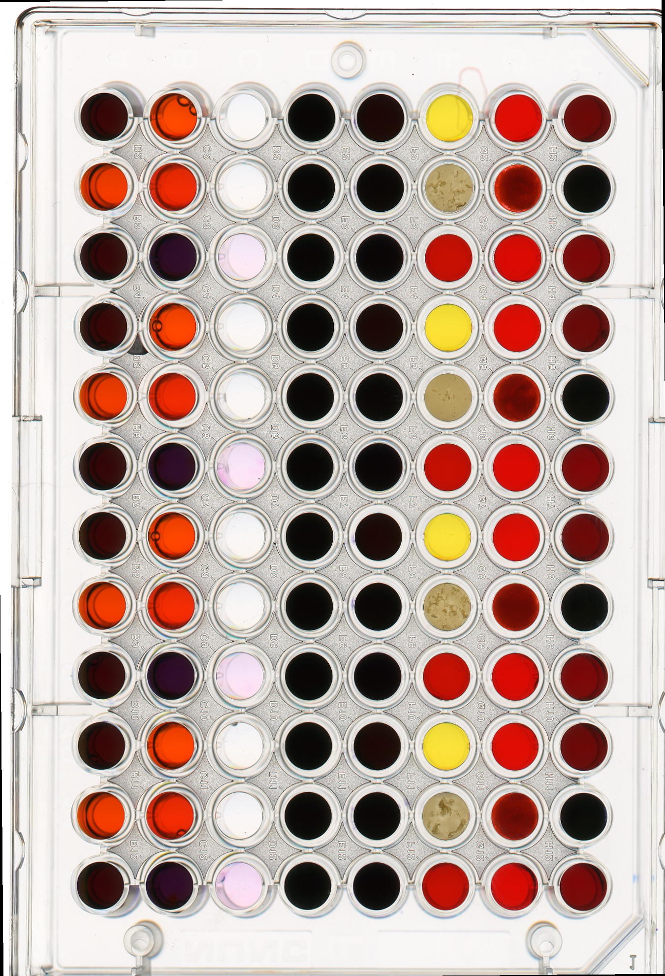
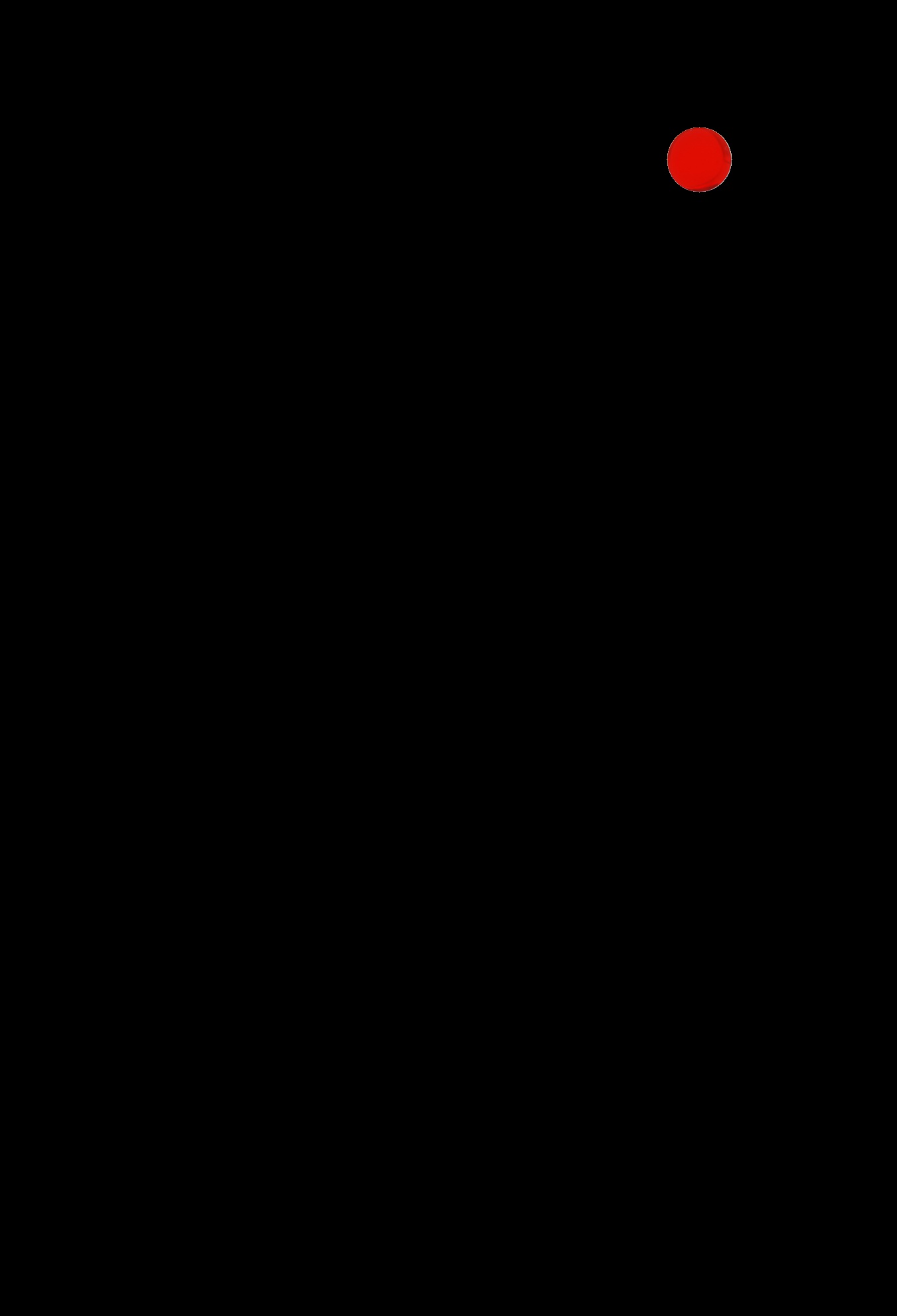
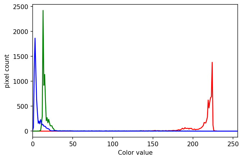
Suppose we are interested in the colour histogram of one of the sensors in the well plate image, specifically, the seventh well from the left in the topmost row, which shows Erythrosin B reacting with water.

Hover over the image with your mouse to find the centre of that well and the radius (in pixels) of the well. Then create a circular mask to select only the desired well. Then, use that mask to apply the colour histogram operation to that well.

Your masked image should look like this:


## Blurring (Giulia)

### Exercise 1: experimenting with sigma values (10 min)

The size and shape of the kernel used to blur an image can have a significant effect on the result of the blurring and any downstream analysis carried out on the blurred image. Try running the code above with a range of smaller and larger sigma values.

#### Generally speaking, what effect does the sigma value have on the blurred image?

### Exercise 2: experimenting with kernel shape (10 min - optional, not included in timing)

Now, what is the effect of applying an asymmetric kernel to blurring an image? Try running the code above with different sigmas in the ry and cx direction. For example, a sigma of 1.0 in the ry direction, and 6.0 in the cx direction.

## Thresholding (Giulia)

### Useful function

def plot_hist(img, bins, x_min, x_max):
    histogram, bin_edges = np.histogram(img, bins, range=(x_min, x_max))

    fig, ax = plt.subplots()
    plt.plot(bin_edges[0:-1], histogram)
    plt.title("Grayscale Histogram")
    plt.xlabel("grayscale value")
    plt.ylabel("pixels")
    plt.xlim(x_min, x_max)

### Exercise 1: more practice with simple thresholding (15 min)

#### First part

Now, it is your turn to practice. Suppose we want to use simple thresholding to select only the coloured shapes (in this particular case we consider grayish to be a colour, too) from the image `data/shapes-02.jpg`.

First, plot the grayscale histogram as in the Creating Histogram episode and examine the distribution of grayscale values in the image. What do you think would be a good value for the threshold t?

#### Second part

Next, create a mask to turn the pixels above the threshold `t` on and pixels below the threshold `t` off. Note that unlike the image with a white background we used above, here the peak for the background colour is at a lower gray level than the shapes. Therefore, change the comparison operator less `<` to greater `>` to create the appropriate mask. Then apply the mask to the image and view the thresholded image. If everything works as it should, your output should show only the coloured shapes on a black background.

### Exercise 2: ignoring more of the images – brainstorming (10 min)

Let us take a closer look at the binary masks produced by the `measure_root_mass` function. You may have noticed in the section on automatic thresholding that the thresholded image does include regions of the image aside of the plant root: the numbered labels and the white circles in each image are preserved during the thresholding, because their grayscale values are above the threshold. Therefore, our calculated root mass ratios include the white pixels of the label and white circle that are not part of the plant root. Those extra pixels affect how accurate the root mass calculation is!

How might we remove the labels and circles before calculating the ratio, so that our results are more accurate? Think about some options given what we have learned so far.

### Exercise 2: ignoring more of the images – implementation (30 min - optional, not included in timing)

Implement an enhanced version of the function measure_root_mass that applies simple binary thresholding to remove the white circle and label from the image before applying Otsu’s method.

### Exercise 3: thresholding a bacteria colony image (15 min)

In the images directory `data/`, you will find an image named `colonies-01.tif`.

This is one of the images you will be working with in the morphometric challenge at the end of the workshop.

1. Plot and inspect the grayscale histogram of the image to determine a good threshold value for the image.
2. Create a binary mask that leaves the pixels in the bacteria colonies “on” while turning the rest of the pixels in the image “off”.

## Connected Component Analysis (Dani)

### Exercise 1:

1. Using the `connected_components` function, find two ways of outputting the number of objects found.
2. Does this number correspond with your expectation? Why/why not?
3. Play around with the `sigma` and `thresh` parameters.
a. How do these parameters influence the number of objects found?
b. OPTIONAL: Can you find a set of parameters that will give you the expected number of objects?

Put your green sticky up when you've finished with 3a

### Exercise 2:

Adjust the `connected_components` function so that it allows `min_area` as an input argument, and only outputs regions above this minimum.

HINT: check out the [skimage.morphology](https://scikit-image.org/docs/stable/api/skimage.morphology.html) library.

BONUS: explore other morphometrics from skimage.measure.regionprops
1. output the centroid position for each object (above the threshold)
2. consider whether you would export or filter by other properties for your own data and/or in what type of images these could be meaningfull

### Capstone Challenge:

In this challenge we will combine a lot of things you have learned over the last few days: blurring, thresholding, masking, connected component analysis, drawing, image formats.

Write a Python function that uses skimage on images of bacterial colonies to:
- count the number of colonies
- calculate their average area
- calculate the total area of all colonies
- show a new image that highlights the colonies
- save this image in a lossless format
- try to put your code into a re-usable function, so that it can be applied conveniently to any image file.

Images can be found in the data folder as colonies-01.tif, colonies-02.tif, and colonies-03.tif.

The final output image should look similar to this:

Don't forget to print the number, average area, and total area of colonies for each image.

BONUS (challenging!): on your output image, highlight the most dense colony by drawing a box around it (i.e., lowest mean pixel value).

## AI and Affine (Bonus Lecture)
###
Bonus Lecture: (Makeda) AI and Affine

Discussion of preparing images for ML:(as per slides)

Exercise 1/1.5: create code to make new_pic1 and new_pic2 augmented images, that are realistic for a Chest Xray machine learning pipeline, then apply what you percieve as the two most critical algorithms to make them ready for classic supervised machine learning in one bit of code.