# A03 - Computing pi
計算$\pi$的方法有很多,我來提供一些其他有趣計算$\pi$的方法
## Fixed-Point Iteration
不知道您有沒有嘗試過在計算機上連續對一個正數連續根號計算,
最後的值會是1

實際上,你可以把它想成是在計算$x = \sqrt{x}$,然後在求x的解是多少,顯然它就是$x = 1$ or $x = 0$
以圖表示的話:

假設我們從$x = 4$開始計算起,那麼

點會朝$x = 1$靠近,因此到最後我們可以取得一個近似解$x = 1 + \epsilon_{x}$,$\epsilon_{x}$為誤差,可惜不會找到解$x = 0$
這個方法被稱為**Fixed-Point Iteration**,就由計算如$x_{i+1} = x_{i} + ...$等形式不斷求得$x$來近似真正解$r$,另外你得自己決定初始項$x_0$是多少
當然並非所有方程式都適合用FPI來解

我們可以使用這個方法來求出$\pi$的近似解
### 求出$\pi$的近似解
首先我們要找出$\pi$的遞迴式
:::info
$0 = \sin{\pi}$
$\Rightarrow \pi = \pi + \sin{(\pi)}$
接下來將$pi$以$x$取代
$\Rightarrow x = x + \sin{(x)}$
$\Rightarrow x_{i+1} = x_i + \sin{(x_i)}$
:::
接下來用$x_{i+1} = x_i + \sin{(x_i)}$來求$\pi$的近似解
```python=
import math
import numpy as np
it = 10 # Iteration
init = 5 # Initial guess
pi = 3.1415926535897932384626433832795028841971 # The real value of pi
f = lambda x : x + math.sin(x) # function handle
data = np.zeros(it)
forward_error = np.zeros(it)
conv_rate = np.zeros(it)
data[0] = init
forward_error[0] = abs(pi - init)
conv_rate[0] = float("nan")
for i in range(1,it) :
data[i] = f(data[i-1])
forward_error[i] = abs(pi - data[i])
if forward_error[i-1] == 0 :
conv_rate[i] = float("nan")
else :
conv_rate[i] = forward_error[i] / forward_error[i-1]
for i in range(it) :
print('Iteration %02d -> x = %.15f, forward error = %.15f, e_{i} / e_{i-1} = %.15f' %( i, data[i], forward_error[i], conv_rate[i]))
```
輸出:
```
Iteration 00 -> x = 5.000000000000000, forward error = 1.858407346410207, e_{i} / e_{i-1} = nan
Iteration 01 -> x = 4.041075725336862, forward error = 0.899483071747069, e_{i} / e_{i-1} = 0.484007488177743
Iteration 02 -> x = 3.258070248108248, forward error = 0.116477594518455, e_{i} / e_{i-1} = 0.129493926208327
Iteration 03 -> x = 3.141855850823108, forward error = 0.000263197233315, e_{i} / e_{i-1} = 0.002259638296988
Iteration 04 -> x = 3.141592653592832, forward error = 0.000000000003039, e_{i} / e_{i-1} = 0.000000011546103
Iteration 05 -> x = 3.141592653589793, forward error = 0.000000000000000, e_{i} / e_{i-1} = 0.000000000000000
Iteration 06 -> x = 3.141592653589793, forward error = 0.000000000000000, e_{i} / e_{i-1} = nan
Iteration 07 -> x = 3.141592653589793, forward error = 0.000000000000000, e_{i} / e_{i-1} = nan
Iteration 08 -> x = 3.141592653589793, forward error = 0.000000000000000, e_{i} / e_{i-1} = nan
Iteration 09 -> x = 3.141592653589793, forward error = 0.000000000000000, e_{i} / e_{i-1} = nan
```
參考圖:

基本上,5個Iteration,準確率可以達小數點後15位,不過很明顯準確率受到浮點數的精度(在Python3.X為小數點後16位)限制
## Newton's method
牛頓法在求解時比起FPI方法有個優勢,牛頓法的收斂會比FPI還要快,因為牛頓法屬於quadratically convergent
$$ M = \lim_{i \rightarrow \infty} \frac{e_{i+1}}{e^2_{i}} < \infty $$
### 推導Newton's method
$f'(x_0) = \frac{0 - f(x_0)}{x - x_0}$
$\Rightarrow x = x_0 - \frac{f(x_0)}{f'(x_0)}$
$\Rightarrow x_{i+1} = x_{i} - \frac{f(x_i)}{f'(x_i)}$
### 求出$\pi$的近似解
已知$0 = sin(\pi)$
令$f(x) = sin(x)$
求$f(x)$的root
然後代入牛頓法,並假設initial guess $x_0 = 3$
$\Rightarrow x_{i+1} = x_i - \frac{\sin{(x_i)}}{\cos{(x_i)}}$
$\Rightarrow x_{i+1} = x_i - \tan{(x_i)}$
```python=
import math
import numpy as np
it = 10 # Iteration
init = 3 # Initial guess
pi = 3.1415926535897932384626433832795028841971 # The real value of pi
f = lambda x : x - math.tan(x) # function handle
data = np.zeros(it)
forward_error = np.zeros(it)
conv_rate = np.zeros(it)
data[0] = init
forward_error[0] = abs(pi - init)
conv_rate[0] = float("nan")
for i in range(1,it) :
data[i] = f(data[i-1])
forward_error[i] = abs(pi - data[i])
if forward_error[i-1] == 0 :
conv_rate[i] = float("nan")
else :
conv_rate[i] = forward_error[i] / math.pow(forward_error[i-1], 2)
for i in range(it) :
print('Iteration %02d -> x = %.15f, forward error = %.15f, e_{i} / e_{i-1}^2 = %.15f' %( i, data[i], forward_error[i], conv_rate[i]))
```
輸出:
```
Iteration 00 -> x = 3.000000000000000, forward error = 0.141592653589793, e_{i} / e_{i-1}^2 = nan
Iteration 01 -> x = 3.142546543074278, forward error = 0.000953889484485, e_{i} / e_{i-1}^2 = 0.047579143449619
Iteration 02 -> x = 3.141592653300477, forward error = 0.000000000289316, e_{i} / e_{i-1}^2 = 0.000317962951472
Iteration 03 -> x = 3.141592653589793, forward error = 0.000000000000000, e_{i} / e_{i-1}^2 = 0.000000000000000
Iteration 04 -> x = 3.141592653589793, forward error = 0.000000000000000, e_{i} / e_{i-1}^2 = nan
Iteration 05 -> x = 3.141592653589793, forward error = 0.000000000000000, e_{i} / e_{i-1}^2 = nan
Iteration 06 -> x = 3.141592653589793, forward error = 0.000000000000000, e_{i} / e_{i-1}^2 = nan
Iteration 07 -> x = 3.141592653589793, forward error = 0.000000000000000, e_{i} / e_{i-1}^2 = nan
Iteration 08 -> x = 3.141592653589793, forward error = 0.000000000000000, e_{i} / e_{i-1}^2 = nan
Iteration 09 -> x = 3.141592653589793, forward error = 0.000000000000000, e_{i} / e_{i-1}^2 = nan
```
## Secant's method
示意圖:
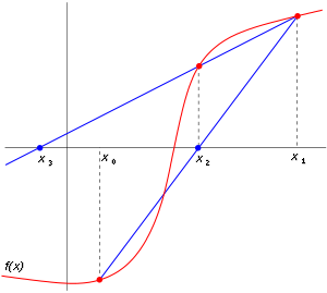
### 推導Secant's method
從Newton's method將$f'(x)$改為$\frac{f(x_i) - f(x_{i-1})}{(x_i - x_{i-1})}$
$\Rightarrow x_{i+1} = x_{i} - \frac{f(x_i)(x_i - x_{i-1})}{(x_i - x_{i-1})}$ for $x_0$ and $x_1$ are initial guess
從方程式中可以發現不必計算$f'(x)$而是改採以$\frac{f(x_i) - f(x_{i-1})}{(x_i - x_{i-1})}$做替代(approximation),在這裡以數值方式取代$f'(x)$
### Error Relationship
$$
e_{i+1} \approx | \frac{f''(r)}{2f'(r)} | e_i e_{i-1}
$$
secant's method的convergence介於linearly convergent與quadratically convergent,屬於superlinear
### 求出$\pi$的近似解
secant's method的定義
```python=
def secant_method(f, x0, x1, k) :
x = np.zeros(k)
x[0] = x0
x[1] = x1
err = np.zeros(k)
err[0] = abs(x0 - pi)
err[1] = abs(x1 - pi)
for i in range(1,k - 1):
if f(x[i]) - f(x[i - 1]) == 0 :
return x, err
x[i + 1] = x[i] - f(x[i]) * (x[i] - x[i - 1]) / (f(x[i]) - f(x[i - 1]))
err[i+1] = abs(x[i+1] - pi)
return x, err
```
```python=
it = 10
pi = 3.1415926535897932384626433832795028841971
f = lambda x : math.sin(x)
data, err = secant_method(f, 3, 4, it)
for i in range(it):
print('Iteration %02d -> x=%.16f, forward error = %.16f' %(i, data[i], err[i]) )
```
輸出:
```
Iteration 00 -> x=3.0000000000000000, forward error = 0.1415926535897931
Iteration 01 -> x=4.0000000000000000, forward error = 0.8584073464102069
Iteration 02 -> x=3.1571627924799470, forward error = 0.0155701388901539
Iteration 03 -> x=3.1394590982180786, forward error = 0.0021335553717146
Iteration 04 -> x=3.1415927279848570, forward error = 0.0000000743950639
Iteration 05 -> x=3.1415926535897367, forward error = 0.0000000000000564
Iteration 06 -> x=3.1415926535897931, forward error = 0.0000000000000000
Iteration 07 -> x=3.1415926535897931, forward error = 0.0000000000000000
Iteration 08 -> x=0.0000000000000000, forward error = 0.0000000000000000
Iteration 09 -> x=0.0000000000000000, forward error = 0.0000000000000000
```
比起Newton's method, secant's method需要更多的iterations才能達到相同的精度,推測是使用以數值解取代以符號運算微分$f(x)$所產生的誤差導致
## False Position Method

### False Position Method推導
把Secant's method做移位整理就可以導出 false position method
$$
c = \frac{bf(a) - af(b)}{f(a) - f(b)}
$$
另外在加上bisection method以$c$更新$a$或$b$
### 求出$\pi$的近似值
False Position Method的定義:
```python=
def false_position_method(f, a, b, k) :
if f(a) * f(b) >= 0 :
raise ValueError('f(a) * f(b) must be < 0')
data = np.zeros(k)
for i in range(k) :
c = (b * f(a) - a * f(b)) / (f(a) - f(b))
data[i] = c
if f(c) == 0 :
return data
if f(a) * f(c) < 0 :
b = c
else :
a = c
return data
```
```python=
it = 10
pi = 3.1415926535897932384626433832795028841971
f = lambda x : math.sin(x)
data = false_position_method(f, 3, 4, it)
for i in range(it):
print('Iteration %02d -> x=%.15f, forward error = %.15f' %(i, data[i], abs(pi - data[i])) )
```
輸出:
```
Iteration 00 -> x=3.157162792479947, forward error = 0.015570138890153
Iteration 01 -> x=3.141546255589150, forward error = 0.000046398000643
Iteration 02 -> x=3.141592655458965, forward error = 0.000000001869172
Iteration 03 -> x=3.141592653589793, forward error = 0.000000000000000
Iteration 04 -> x=3.141592653589793, forward error = 0.000000000000000
Iteration 05 -> x=3.141592653589793, forward error = 0.000000000000000
Iteration 06 -> x=3.141592653589793, forward error = 0.000000000000000
Iteration 07 -> x=3.141592653589793, forward error = 0.000000000000000
Iteration 08 -> x=3.141592653589793, forward error = 0.000000000000000
Iteration 09 -> x=3.141592653589793, forward error = 0.000000000000000
```
## Inverse Quadratic Interpolation
$$
x_{i+3} = x{i+2} - \frac{r(r - q)(c - b) + (1 - r)s(c - a)}{(q - 1)(r - 1)(s - 1)}
$$
where $a = x_i, b = x_{i+1}, c = x_{i+2}$ and $q = \frac{f(a)}{f(b)}$, $r = \frac{f(c)}{f(b)}$, and $s = \frac{f(c)}{f(a)}$
## Pros & Cons
### 優勢
- 比起使用Leibniz formula與Monte Carlo Method,只需要較少的iterations就可以達到相同精度的$\pi$,也不需要取樣
- 方程式簡單,只需要計算sin與tan與x相加減就可以完成一次Iteration計算,因此計算效率與精度取決於sin與tan實作
- 精度隨著iteration增加而上升,因此很適合用於time-sensitived系統或是real-time系統
### 缺點
- 很顯然地,精確度限於浮點數,因此若要更大精確度必須重新實作更高精確度的浮點數機制以及sin與tan的實作
- sin與tan的實作成為效率關鍵
## 參考資料
- Sauer - Numerical Analysis , 2nd Edition
 Sign in with Wallet


