# 用 R 配適邏輯式族群生長曲線
###### tags: `用R做` `生態學`

高中生物課本告訴我們，若不考慮環境限制因子，一個生物族群的規模隨著時間會呈現指數式成長；而現實情況中因為資源有限，所以實際上的族群量會有個上限，那個上線就是環境負載量。

大學生態學課本裡，會用數學式子來表示。對於沒有任何限制，且大小為 $N$ 的族群，在 $t$ 時間區段的增長速度 $\frac{\mathrm{d}N}{\mathrm{d}t}=rN$，可以發現平均速度（per capita rate of increase）$r$ 為定值，跟族群數量無關，所以隨著時間過去，族群數量會直直衝，在族群大小—時間圖上形成 **J 形曲線**，表示為 $N_t=N_0\times(1+r)^t$。。
不過現實上，因為有環境負載量，所以實際上的量測的族群成長速率會是$\frac{\mathrm{d}N}{\mathrm{d}t}=r\left(\frac{K-N}{N}\right)N$，比指數成長曲線的速率多了$\left(\frac{K-N}{N}\right)$一項，其中 $K$ 就是環境承載量（carrying capacity）。當族群數量與環境承載量相當時，族群成長速率趨近於 0。考慮環境負載量的族群成長曲線會近似於邏輯式曲線（logistic curve），通式為：$N_t=\frac{N_0Ke^{rt}}{N_0(e^{rt}-1)+K}=\frac{K}{1+\left(\frac{K-P_0}{N_0}\right)e^{-rt}}$；隨時間過去，族群量會越來越近似於環境負載量：$\lim\limits_{t \to \inf}N_t=K$，最後在族群大小—時間圖上形成 **S 形曲線**。

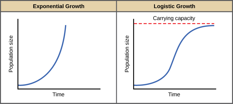
取自[BioNinjia](https://ib.bioninja.com.au/options/option-c-ecology-and-conser/c5-population-ecology/population-growth.html)

---
## 如何配適不同種類的族群成長曲線
如果手上有不同時間調查的族群量資料，要怎麼配適（fit）不同的成長曲線呢？
如果要配適指數曲線，那很容易，在 R 當中只需要先使用 `log()` 函數，將時間與族群數量都取自然對數，那麼原本的指數成長函式，就會成為一個 $y=b+ax$ 形式的二元一次函式，此時使用 `lm()` 函數，就可以做簡單線性迴歸了。

困難的是如何配是邏輯式迴歸曲線。

我們一樣可以使用類似的思維，並且利用 R 的 `car` 套件中 `logit()` 函數，把族群量做邏輯式轉換。如此一來，就可以取得邏輯式函數中的幾個重要參數作為非線性迴歸分析的初始值。
要注意邏輯式迴歸的通式為 $f(x)=\frac{L}{1+e^{-k(x-x_0)}}$，且輸入 `logit()` 函數的數值必須介於 0–100，若族群數量大，需要先進行縮放。

接著，就讓我們以一組由真實測量值改編而來的數據，在 R 裡面來實作吧：

data <- data.frame(Year = c(2001,2002,2004,2007,2008,2011,2012,2014,2015,2016,2017,2018,2019,2020,2021),
                   Population = c(4286,12345,24376,32054,54849,71539,125486,249867,347659,442693,426483,413752,436859,436281,406748))

#先求取邏輯式轉換後的族群量，與年份做簡單線性迴歸
coef(lm(car::logit(Population/10000) ~ Year, data = data))

#輸出值如下
> coef(lm(car::logit(Population/10000) ~ Year, data = data))
Note: largest value of p > 1 so values of p interpreted as percents
(Intercept)        Year 
 -522.68343     0.25882 

取得初始值之後，使用 `nls()` 函數進行非線性迴歸分析。在函數中可以自行設定要用來配適的式子，並且提供參數初始值，讓 R 以 [Gauss-Newton 最佳化演算法](https://en.wikipedia.org/wiki/Gauss%E2%80%93Newton_algorithm)自動尋找最適合的參數組合。

#按照簡單線性迴歸的值填入初始值進行參數估計
logfit <- nls((Population/10000) ~ L/(1 + exp(-k - k0 * Year)),
              start = list(L = 43, k = -522.6834, k0 = 0.2588), data = data, trace = TRUE)

因為設定了 `trace = T`，在尋找最佳參數組時，會印出過程。最後也可以用 `summary()` 看到最適合的配適報表：

#會顯示過程
4670.068    (6.06e+00): par = (43 -522.6834 0.2588)
4441.872    (6.41e+00): par = (33.92782 -568.865 0.2819435)
3914.072    (6.26e+00): par = (27.31519 -675.0361 0.334958)
2553.880    (4.91e+00): par = (27.19346 -904.6359 0.4492841)
738.6889    (2.65e+00): par = (34.44295 -1247.975 0.6199525)
87.36834    (6.09e-02): par = (43.83912 -1500.953 0.7455575)
86.97634    (1.41e-02): par = (43.81089 -1535.034 0.762475)
86.95533    (3.08e-03): par = (43.80457 -1543.508 0.7666821)
86.95432    (6.64e-04): par = (43.80379 -1545.252 0.7675478)
86.95428    (1.44e-04): par = (43.80346 -1545.653 0.7677465)
86.95427    (3.02e-05): par = (43.80342 -1545.735 0.7677875)
86.95427    (8.44e-06): par = (43.80341 -1545.753 0.7677962)    

> summary(logfit)

Formula: (Population/10000) ~ L/(1 + exp(-k - k0 * Year))

Parameters:
     Estimate Std. Error t value Pr(>|t|)    
L     43.8034     1.4543  30.121 1.12e-12 ***
k  -1545.7527   237.6781  -6.504 2.92e-05 ***
k0     0.7678     0.1181   6.503 2.93e-05 ***
---
Signif. codes:  0 ‘***’ 0.001 ‘**’ 0.01 ‘*’ 0.05 ‘.’ 0.1 ‘ ’ 1

Residual standard error: 2.692 on 12 degrees of freedom

Number of iterations to convergence: 11 
Achieved convergence tolerance: 8.439e-06

最後就可以開心出圖了：

library(ggplot2)
L <- coef(logfit)[1] *10000
k <- coef(logfit)[2]
k0 <- coef(logfit)[3]

#製作繪製配適函數用的數據
x <- seq(min(data$Year), max(data$Year), length = 200)
y <- L/(1 + exp(-k - k0 * x))
predict <- data.frame(x, y)

ggplot(data = data, aes(x = Year, y = Population)) +
  geom_line(data = predict, aes(x = x, y = y), size = 1) +
  geom_point(color = "blue",size = 4) +
  labs(x = "Year", y = "Estimated population size") +
  scale_x_continuous(breaks = seq(2000, 2022, 2)) +
  scale_y_continuous(labels = scales::comma) +
  theme_bw() +
  theme(axis.text = element_text(size = 12), 
        axis.title = element_text(size = 16),
        panel.grid.minor = element_blank())

如此就可以繪出實際的調查結果（藍點）與配適的函數（黑線）。


## 如果不想自己餵初始參數......
如果覺得要先做線性迴歸當成初始參數實在太麻煩，或者不想多呼叫一個套件，也可以使用內建的 `SSlogis` 參數直接做非線性迴歸：

autofit <- nls(Population ~ SSlogis(Year, L, k, k0), data = data)
> summary(autofit)

Formula: Population ~ SSlogis(Year, L, k, k0)

Parameters:
    Estimate Std. Error  t value Pr(>|t|)    
L  4.380e+05  1.454e+04   30.121 1.12e-12 ***
k  2.013e+03  2.482e-01 8111.057  < 2e-16 ***
k0 1.302e+00  2.003e-01    6.503 2.93e-05 ***
---
Signif. codes:  0 ‘***’ 0.001 ‘**’ 0.01 ‘*’ 0.05 ‘.’ 0.1 ‘ ’ 1

Residual standard error: 26920 on 12 degrees of freedom

Number of iterations to convergence: 1 
Achieved convergence tolerance: 3.803e-06

在這個功能中，就不需要把族群數量轉換到 100 以內了。
接下來一樣畫個圖來看看：

L.n <- coef(autofit)[1]
k.n <- coef(autofit)[2]
k0.n <- coef(autofit)[3]
x.n <- seq(min(data$Year), max(data$Year), length = 200) #construct a range of x values bounded by the data
y.n <- L.n/(1 + exp((x.n - k.n) * -k0.n)) #predicted mass
predict.n <- data.frame(x.n, y.n)
ggplot(data = data, aes(x = Year, y = Population)) +
  geom_line(data = predict.n, aes(x = x.n, y = y.n), size = 1) +
  geom_point(color = "blue",size = 4) +
  labs(x = "Year", y = "Estimated population size") +
  scale_x_continuous(breaks = seq(2000, 2022, 2)) +
  scale_y_continuous(labels = scales::comma) +
  theme_bw() +
  theme(axis.text = element_text(size = 12), 
        axis.title = element_text(size = 16),
        panel.grid.minor = element_blank())


可以發現使用 `SSlogis()` 功能配適出的函數，在曲線左側的配適效果不太好。
比較兩種結果，顯然我們手動用簡單線性迴歸產出初始值來適配的結果好一些，所以之後要進行類似的適配，還是多做一個步驟吧。若想了解如何把配式出的方程式印到圖上，可以參考[如何印出方程式與統計量到ggplot圖上](/kuuMAB8tSuukIOD9fxAuDQ)。
圖片來自[此](https://www.appstate.edu/~whiteheadjc/service/logit/intro.htm)

#### 參考資料與延伸閱讀
1. Cramer, J. S. (2003). [The origins and development of the logit model](https://www.cambridge.org/resources/0521815886/1208_default.pdf). *Logit models from economics and other fields*, 2003, 1-19.
2. [Logistic Equation](https://mathworld.wolfram.com/LogisticEquation.html)

<span style="font-size:30px">🐕‍🦺</span><font color="dcdcdc">2023.10.22</font>