# Getting Started with Prometheus and TimescaleDB using Promscale
## Introduction
[Prometheus][prometheus-webpage] is an open-source systems monitoring and alerting toolkit that can be used to easily and cost-effectively monitor infrastructure and applications. Over the past few years, Prometheus has emerged as the monitoring solution for modern software systems. The key to Prometheus’ success is its pull-based architecture and service discovery, which is able to seamlessly monitor modern, dynamic systems in which (micro-)services startup and shutdown frequently.
**The Problem: Prometheus is not designed for analytics**
As organizations use Prometheus to collect data from more and more of their infrastructure, the benefits from mining this data also increase. Analytics becomes critical for auditing, reporting, capacity planning, prediction, root-cause analysis, and more. Prometheus's architectural philosophy is one of simplicity and extensibility. Accordingly, it does not itself provide durable, highly-available long-term storage or advanced analytics, but relies on other projects to implement this functionality.
There are existing ways to durably store Prometheus data, but while these options are useful for long-term storage, they only support the Prometheus data model and query model (limited to the PromQL query language). While these work extremely well for the simple, fast analyses found in dashboarding, alerting, and monitoring, they fall short for more sophisticated analysis capabilities, or for the ability to enrich their dataset with other sources needed for insight-generating cross-cutting analysis.
**Solution: Promscale scales and augments Prometheus for long-term storage and analytics**
[Promscale][promscale-github] is an open-source long-term store for Prometheus data, designed for analytics. It is a horizontally scalable and operationally mature platform for Prometheus data. Promscale offers the combined power of PromQL and SQL, enabling you to ask any question, create any dashboard, and achieve greater visibility into your systems.
Promscale is built on top of TimescaleDB, the leading relational database for time-series. Promscale also supports native compression, handles high-cardinality, provides rock-solid reliability, and more. Furthermore, it offers other native time-series capabilities, such as data retention policies, continuous aggregate views, downsampling, data gap-filling, and interpolation. It is already natively supported by Grafana via the Prometheus and PostgreSQL/TimescaleDB data sources.
> :TIP: For an overview of Promscale, see this short introductory video: [Intro to Promscale - Advanced analytics for Prometheus][promscale-intro-video].
In this document, you will learn:
1. The benefits of using Promscale to store and analyze Prometheus metrics
2. How Promscale works
3. How to install Prometheus, Promscale and TimescaleDB
4. How to run queries in PromQL and SQL against Promscale
## 1. Why use Promscale & TimescaleDB to store Prometheus metrics [](why-promscale)
This section details five reasons to use Timescale and Promscale to store Prometheus metrics:
1. Long term data storage
2. Operational ease
3. Queries in SQL and PromQL
4. Per Metric Retention
5. Ability to push data from custom applications
### 1.1 Long term data storage
In order to keep Prometheus simple and easy to operate, its creators intentionally left out many scaling features one would normally expect. Data in Prometheus is stored locally within the instance and is not replicated. Having both compute and data storage on one node may make it easier to operate, but also makes it harder to scale and ensure high availability.
As a result, Prometheus is not designed to be a long-term metrics store. From the [documentation][prometheus storage docs]:
>Prometheus is not arbitrarily scalable or durable in the face of disk or node outages and should thus be treated as more of an ephemeral sliding window of recent data.
On the other hand, TimescaleDB can easily handle petabytes of data, and supports high availability and replication, making it a good fit for long term data storage. In addition, it provides advanced capabilities and features, such as full SQL, JOINs and data retention and aggregation policies, all of which are not available in Prometheus.
Using Promscale as a long term store for Prometheus metrics works as follows:
* All metrics that are scraped from targets are first written to the Prometheus local storage.
* Metrics are then written to Promscale via the Prometheus `remote-write` endpoint.
* This means that all of your metrics are ingested in parallel to TimescaleDB using Promscale, making any Prometheus disk failure less painful.
TimescaleDB can also store other types of data (metrics from other systems, time-series data, relational data, metadata), allowing you to consolidate monitoring data from different sources into one database and simplify your stack. You can also join different types of data and add context to your monitoring data for richer analysis, using SQL `JOIN`s.
Moreover, the recent release of [TimescaleDB 2.0][multinode-blog] introduces multi-node functionality, making it easier to scale horizontally and store data at petabyte scale.
### 1.2 Operational ease
Promscale is an exception. Promscale operates as a single stateless service. This means that once you configure the `remote-write` & `remote-read` endpoints in your prometheus configuration file then all samples forwarded to Promscale. Promscale then handles the ingestion of samples into TimescaleDB. Promscale exposes all Prometheus compatible APIs, allowing you to query Promscale using PromQL queries.
Moreover, the only way to scale Prometheus is by [federation][prometheus-federation]. However, there are cases where federation is not a good fit: for example, when copying large amounts of data from multiple Prometheus instances to be handled by a single machine. This can result in poor performance, decreased reliability (an additional point of failure), and loss of some data. These are all problems you can avoid by using an operationally simple and mature platform like Promscale combined with TimescaleDB.
Furthermore, with Promscale, it's simple to get a global view of all metrics data, using both PromQL and SQL queries.
### 1.3 Queries in SQL and PromQL
By allowing a user to use SQL, in addition to PromQL, Promscale empowers the user to ask complex analytical queries from their metrics data, and thus extract more meaningful insights.
PromQL is the Prometheus native query language. It’s a powerful and expressive query language that allows you to easily slice and dice metrics data and use a variety of monitoring specific [functions][promql-functions].
However, there may be times where you need greater query flexibility and expressiveness than what PromQL provides. For example, trying to cross-correlate metrics with events and incidents that occurred, running more granular queries for active troubleshooting, or applying machine learning or other forms of deeper analysis on metrics.
TimescaleDB's full SQL support is of great help in these cases. It enables you to apply the full breadth of SQL to your Prometheus data, joining your metrics data with any other data you might have, and run more powerful queries.
We detail examples of such SQL queries in Part 4 of this tutorial.
### 1.4 Per Metric Retention
Promscale maintains isolation between metrics. This allows you to set retention periods, downsampling and compression settings on a per metric basis, giving you more control over your metrics data.
Per metric retention policies, downsampling, aggregation and compression helps you store only series you care about for the long term. This helps you better trade off the value brought by keeping metrics for the long term with the storage costs involved, allowing you to keep metrics that matter for as long as you need and discarding the rest to save on costs.
This isolation extends to query performance, wherein queries for one metric are not affected by the cardinality or query and write load of other metrics. This provides better performance on smaller metrics and in general provides a level of safety within your metric storage system.
### 1.5 Ability to push data from custom applications
The Promscale write endpoints also accept data from your custom applications (i.e data outside of Prometheus) in JSON format.
All you have to do is parse your existing time series data to object format below:
```
{
"labels":{"__name__": "cpu_usage", "namespace":"dev", "node": "brain"},
"samples":[
[1577836800000, 100],
[1577836801000, 99],
[1577836802000, 98],
...
]
}
```
Then perform a write request to Promscale:
```
curl --header "Content-Type: application/json" \
--request POST \
--data '{"labels":{"__name__":"foo"},"samples":[[1577836800000, 100]]}' \
"http://localhost:9201/write"
```
For more details on writing custom time-series data to Promscale can be found in this document: [Writing to Promscale][Writing TO Promscale]
## 2. How Promscale Works [](how-to)
### 2.1 Promscale Architecture
Unlike some other long-term data stores for Prometheus, the basic Promscale architecture consists of only three components: Prometheus, Promscale, and TimescaleDB.
The diagram below explains the high level architecture of Promscale, including how it reads and writes to Prometheus, and how it can be queried by additional components, like PromLens, Grafana and any other SQL tool.
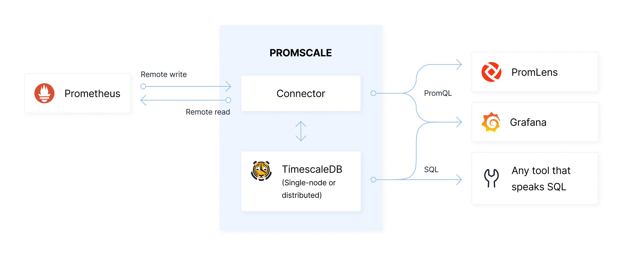
**Ingesting metrics**
* Once installed alongside Prometheus, Promscale automatically generates an optimized schema which allows you to efficiently store and questy your metrics using SQL.
* Prometheus will write data to the Connector using the Prometheus`remote_write` interface.
* The Connector will then write data to TimescaleDB.
**Querying metrics**
* PromQL queries can be directed to the Connector, or to the Prometheus instance, which will read data from the Connector using the `remote_read` interface. The Connector will, in turn, fetch data from TimescaleDB.
* SQL queries are handled by TimescaleDB directly.
As can be seen, this architecture has relatively few components, enabling simple operations.
**Promscale PostgreSQL Extension**
Promscale has a dependency on the [Promscale PostgreSQL extension][promscale-extension], which contains support functions to improve the performance of Promscale. While Promscale is able to run without the additional extension installed, adding this extension will get better performance from Promscale.
**Deploying Promscale**
Promscale can be deployed in any environment running Prometheus, alongside any Prometheus instance. We provide Helm charts for easier deployments to Kubernetes environments (see Section 3 of this tutorial for more on installation and deployment).
### 2.2 Promscale Schema
To achieve high ingestion, query performance and optimal storage we have designed a schema which takes care of writing the data in the most optimal format for storage and querying in TimescaleDB. Promscale translates data from the [Prometheus data model][Prometheus native format] into a relational schema that is optimized for TimescaleDB, is stored efficiently, and is easy to query.
The basic schema uses a normalized design where the time-series data is stored in compressed hypertables. These tables have a foreign-key to series tables (stored as vanilla PostgreSQL tables), where each series consists of a unique set of labels.
In particular, this schema decouples individual metrics, allowing for the collection of metrics with vastly different cardinalities and retention periods. At the same time, Promscale exposes simple, user-friendly views so that you do not have to understand this optimized schema (see 2.3 for more on views).
> :TIP: Promscale automatically creates and manages database tables. So, while understanding the schema can be beneficial (and interesting), it is not required to use Promscale. Skip to Section 2.3 for information how to interact with Promscale using SQL views and to Section 4 to learn using hands on examples.
#### 2.2.1 Metrics Storage Schema
Each metric is stored in a separate hypertable.
A hypertable is a TimescaleDB abstraction that represents a single logical SQL table that is automatically physically partitioned into chunks, which are physical tables that are stored in different files in the filesystem. Hypertables are partitioned into chunks by the value of certain columns. In this case, we will partition out tables by time (with a default chunk size of 8 hours).
**Compression**
The first chunk will be decompressed to serve as a high-speed query cache. Older chunks are stored as compressed chunks. We configure compression with the segment_by column set to the series_id and the orderby column set to time DESC. These settings control how data is split into blocks of compressed data. Each block can be accessed and decompressed independently.
The settings we have chosen mean that a block of compressed data is always associated with a single series_id and that the data is sorted by time before being split into blocks; thus each block is associated with a fairly narrow time range. As a result, in compressed form, accesses by series_id and time range are optimized.
**Example**
The hypertables for each metric use the following schema (using `cpu_usage` as an example metric):
The `cpu_usage` table schema:
```sql=
CREATE TABLE cpu_usage (
time TIMESTAMPTZ,
value DOUBLE PRECISION,
series_id BIGINT,
)
CREATE INDEX ON cpu_usage (series_id, time) INCLUDE (value)
```
```sql
Column | Type | Modifiers
-----------+--------------------------+-----------
time | TIMESTAMPTZ |
value | DOUBLE PRECISION |
series_id | BIGINT |
```
In the above table, `series_id` is foreign key to the `series` table described below.
#### 2.2.2 Series Storage Schema
Conceptually, each row in the series table stores a set of key-value pairs.
In Prometheus such a series is represented as a one-level JSON string. For example: `{ “key1”:”value1”, “key2”:”value2”}`. But the strings representing keys and values are often long and repeating. So, to save space, we store a series as an array of integer “foreign keys” to a normalized labels table.
The definition of these two tables is shown below:
``` sql
CREATE TABLE _prom_catalog.series (
id serial,
metric_id int,
labels int[],
UNIQUE(labels) INCLUDE (id)
);
CREATE INDEX series_labels_id ON _prom_catalog.series USING GIN (labels);
CREATE TABLE _prom_catalog.label (
id serial,
key TEXT,
value text,
PRIMARY KEY (id) INCLUDE (key, value),
UNIQUE (key, value) INCLUDE (id)
);
```
### 2.3 Promscale Views
The good news is that in order to use Promscale well, you do not need to understand the schema design. Users interact with Prometheus data in Promscale through views. These views are automatically created and are used to interact with metrics and labels.
Each metric and label has its own view. You can see a list of all metrics by querying the view named `metric`. Similarly, you can see a list of all labels by querying the view named `label`. These views are found in the `prom_info` schema.
### Metrics Information View
Querying the `metric` view returns all metrics collected by Prometheus:
```
SELECT *
FROM prom_info.metric;
```
Here is one row of a sample output for the query above:
```
id | 16
metric_name | process_cpu_seconds_total
table_name | process_cpu_seconds_total
retention_period | 90 days
chunk_interval | 08:01:06.824386
label_keys | {__name__,instance,job}
size | 824 kB
compression_ratio | 71.60883280757097791800
total_chunks | 11
compressed_chunks | 10
```
Each row in the `metric` view, contains fields with the metric `id`, as well as information about the metric, such as its name, table name, retention period, compression status, chunk interval etc.
Promscale maintains isolation between metrics. This allows users to set retention periods, downsampling and compression settings on a per metric basis, giving users more control over their metrics data.
### Labels Information View
Querying the `label` view returns all labels associated with metrics collected by Prometheus:
```
SELECT *
FROM prom_info.label;
```
Here is one row of a sample output for the query above:
```
key | collector
value_column_name | collector
id_column_name | collector_id
values | {arp,bcache,bonding,btrfs,conntrack,cpu,cpufreq,diskstats,edac,entropy,filefd,filesystem,hwmon,infiniband,ipvs,loadavg,mdadm,meminfo,netclass,netdev,netstat,nfs,nfsd,powersupplyclass,pressure,rapl,schedstat,sockstat,softnet,stat,textfile,thermal_zone,time,timex,udp_queues,uname,vmstat,xfs,zfs}
num_values | 39
```
Each label row contains information about a particular label, such as the label key, the label's value column name, the label's id column name, the list of all values taken by the label and the total number of values for that label.
For examples of querying a specific metric view, see Section 4 of this tutorial.
## 3. Up and Running: Install Prometheus, Promscale and TimescaleDB [](up-and-running)
We recommend four methods to setup and install Promscale:
1. [TOBS - The Observability Stack for Kubernetes ][tobs-github] (recommended for kubernetes deployments)
2. Docker (instructions detailed below)
3. [Helm][promscale-helm-chart]
4. [Bare Metal][promscale-baremetal-docs]
> :TIP: See the [Promscale github installation guide][promscale-github-installation] for more information on installation options.
For demonstration purposes, we will use Docker to get up and running with Promscale.
The easiest way to get started is by using Docker images. Make sure you have Docker installed on your local machine ([Docker installation instructions][docker]).
The instructions below have 4 steps:
1. Install TimescaleDB
2. Install Prometheus
3. Install Promscale
4. Install node_exporter
>:WARNING: The instructions below are local testing purposes only and should not be used to set up a production environment.
### Step 1: Install TimescaleDB
First, let's create a network specific to Promscale and TimescaleDB:
```docker network create --driver bridge promscale-timescaledb```
Secondly, let's install and spin up an instance of TimescaleDB in a docker container. This is where Promscale will store all metrics data scraped from Prometheus targets.
We will use a docker image which has the`promscale` PostgreSQL extension already pre-installed:
```bash
docker run --name timescaledb \
--network promscale-timescaledb \
-e POSTGRES_PASSWORD=<password> -d -p 5432:5432 \
timescaledev/timescaledb-ha:pg12-latest
```
The above commands creates a TimescaleDB instanced named `timescaledb` (via the `--name` flag), on the network named `promscale-timescale` (via the `--network` flag), whose container will run in the background with the container ID printed after created (via the `-d` flag), with port-forwarding it to port `5432` on your machine (via the `-p` flag).
> :WARNING: Note we set the `POSTGRES_PASSWORD` environment variable (using the `-e` flag) in the command above. Please ensure to replace `<password>` with the password of your choice for the `postgres` superuser.
>
> Note that for production deployments, you will want to fix the docker tag to a particular version instead of `pg12-latest`
### Step 2: Install Promscale
Since we have TimescaleDB up and running, let’s spin up a [Promscale][promscale-github], using the [Promscale docker image][promscale-docker-image] available on Docker Hub:
```bash
docker run --name promscale -d -p 9201:9201 \
--network promscale-timescaledb \
timescale/promscale:latest
-db-uri postgres://postgres:<password>@timescaledb:5432/postgres?sslmode=allow
```
In the `-db-uri` flag above, the second mention of `postgres` refers the the user we're logging into the database as, `<password>` is the password for user `postgres` and `timescaledb` is the name of the TimescaleDB container, installed in step 1. We can use the name `timescaledb` to refer to the database, rather than using its host address, as both containers are on the same docker network `promscale-timescaledb`.
>**:WARNING: Note**: The setting `ssl-mode=allow` is for testing purposes only. For production deployments, we advise you to use `ssl-mode=require` for security purposes.
>
> Furthermore, note that value`<password>` should be replaced with the password you set up for TimescaleDB in step 1 above.
### Step 3: Start collecting metrics using node_exporter
`node_exporter` is a Prometheus exporter for hardware and OS metrics exposed by *NIX kernels, written in Go with pluggable metric collectors. To learn more about it, refer to the [Node Exporter Github][].
For the purposes of this tutorial, we need a service that will expose metrics to Prometheus. We will use the `node_exporter` for this purpose.
Install the the `node_exporter` on your machine by running the docker command below:
```bash
docker run --name node_exporter -d -p 9100:9100 \
--network promscale-timescaledb \
quay.io/prometheus/node-exporter
```
The command above creates a node exporter instanced named `node_exporter`, which port-forwards its output to port `9100` and runs on the `promscale-timescaledb` network created in Step 1.
Once the Node Exporter is running, you can verify that system metrics are being exported by visiting its `/metrics` endpoint at the following URL: `http://localhost:9100/metrics`. Prometheus will scrape this `/metrics` endpoint to get metrics.
### Step 4: Install Prometheus
All that's left is to spin up Prometheus.
First we need to ensure that our Prometheus configuration file `prometheus.yml` is pointing to Promscale and that we’ve properly set the scrape configuration target to point to our `node_exporter` instance, created in Step 3.
Here is a basic `prometheus.yml` configuration file that we'll use for this tutorial. ([More information on Prometheus configuration][first steps])
**A basic `prometheus.yml` file for Promscale:**
```yaml
global:
scrape_interval: 10s
evaluation_interval: 10s
scrape_configs:
- job_name: prometheus
static_configs:
- targets: ['localhost:9090']
- job_name: node-exporter
static_configs:
- targets: ['node_exporter:9100']
remote_write:
- url: "http://promscale:9201/write"
remote_read:
- url: "http://promscale:9201/read"
read_recent: true
```
In the file above, we configure Prometheus to use Promscale as its remote storage endpoint by pointing both its `remote_read` and `remote_write` to Promscale URLs. Moreover, we set node-exporter as our target to scrape every 10s.
Next, let's spin up a Prometheus instance using the configuration file above (assuming it's called `prometheus.yml` and is in the current working directory), using the following command:
```bash
docker run \
--network promscale-timescaledb \
-p 9090:9090 \
-v ${PWD}/prometheus.yml:/etc/prometheus/prometheus.yml \
prom/prometheus
```
### BONUS: Docker Compose File
To save time spinning up and running each docker container separately, here is a sample`docker-compose.yml` file that will spin up docker containers for TimescaleDB, Promscale, node_exporter and Prometheus using the configurations mentioned in Steps 1-4 above.
> :WARNING: Ensure you have the Prometheus configuration file `prometheus.yml` in the same directory as `docker-compose.yml`)
**A sample `docker-compose.yml` file to spin up and connect TimescaleDB, Promscale, node_exporter and Prometheus:** is available in the [Promscale Github repo][promscale-docker-compose].
To use the docker-compose file above method, follow these steps:
1. In `docker-compose.yml`, set `<PASSWORD>`, the password for superuser `postgres` in TimescaleDB, to a password of your choice.
2. Run the command `docker-compose up` in the same directory as the `docker-compose.yml` file .
3. That's it! TimescaleDB, Promscale, Prometheus, and node-exporter should now be up and running.
Now you're ready to run some queries!
## 4. Running queries using Promscale
Promscale offers the combined power of PromQL and SQL, enabling you to ask any question, create any dashboard, and achieve greater visibility into the systems you monitor.
In the configuration used in Part 3 above, Prometheus will scrape the Node Exporter every 10s and metrics will be stored in both Prometheus and TimescaleDB, via Promscale.
This section will illustrate how to run simple and complex SQL queries against Promscale, as well as queries in PromQL.
### 4.1 SQL Queries in Promscale
You can query Promscale in SQL from your favorite favorite SQL tool or using psql:
```bash
docker exec -it timescaledb psql postgres postgres
```
The above command first enters our timescaledb docker container (from Step 3.1 above) and creates an interactive terminal to it. Then it opens up`psql`, a terminal-based front end to PostgreSQL (More information on psql -- [psql docs][].
Once inside, we can now run SQL queries and explore the metrics collected by Prometheus and Promscale
**4.1.1 Querying a metric:**
Queries on metrics are performed by querying the view named after the metric you're interested in.
In the example below, we will query a metric named `go_dc_duration` for its samples in the past 5 minutes. This metric is a measurement for how long garbage collection is taking in Golang applications:
``` sql
SELECT * from go_gc_duration_seconds
WHERE time > now() - INTERVAL '5 minutes';
```
Here is a sample output for the query above (your output will differ):
```
time | value | series_id | labels | instance_id | job_id | quantile_id
----------------------------+-------------+-----------+-------------------+-------------+--------+-------------
2021-01-27 18:43:42.389+00 | 0 | 495 | {208,43,51,212} | 43 | 51 | 212
2021-01-27 18:43:42.389+00 | 0 | 497 | {208,43,51,213} | 43 | 51 | 213
2021-01-27 18:43:42.389+00 | 0 | 498 | {208,43,51,214} | 43 | 51 | 214
2021-01-27 18:43:42.389+00 | 0 | 499 | {208,43,51,215} | 43 | 51 | 215
2021-01-27 18:43:42.389+00 | 0 | 500 | {208,43,51,216} | 43 | 51 | 216
```
Each row returned contains a number of different fields:
* The most important fields are `time`, `value` and `labels`.
* Each row has a `series_id` field, which uniquely identifies its measurements label set. This enables efficient aggregation by series.
* Each row has a field named `labels`. This field contains an array of foreign key to label key-value pairs making up the label set.
* While the `labels` array is the entire label set, there are also seperate fields for each label key in the label set, for easy access. These fields end with the suffix `_id` .
**4.1.2 Querying values for label keys**
As explained in the last bullet point above, each label key is expanded out into its own column storing foreign key identifiers to their value, which allows us to JOIN, aggregate and filter by label keys and values.
To get back the text represented by a label id, use the `val(field_id)` function. This opens up nifty possibilities such as aggregating across all series with a particular label key.
For example, take this example, where we find the median value for the `go_gc_duration_seconds` metric, grouped by the job associated with it:
``` sql
SELECT
val(job_id) as job,
percentile_cont(0.5) within group (order by value) AS median
FROM
go_gc_duration_seconds
WHERE
time > now() - INTERVAL '5 minutes'
GROUP BY job_id;
```
Sample Output:
```
job | median
---------------+-----------
prometheus | 6.01e-05
node-exporter | 0.0002631
```
**4.1.3 Querying label sets for a metric**
As explained in Section 2, the `labels` field in any metric row represents the full set of labels associated with the measurement and is represented as an array of identifiers.
To return the entire labelset in JSON, we can apply the `jsonb()` function, as in the example below:
``` sql
SELECT
time, value, jsonb(labels) as labels
FROM
go_gc_duration_seconds
WHERE
time > now() - INTERVAL '5 minutes';
```
Sample Output:
```sql
time | value | labels
----------------------------+-------------+----------------------------------------------------------------------------------------------------------------------
2021-01-27 18:43:48.236+00 | 0.000275625 | {"job": "prometheus", "__name__": "go_gc_duration_seconds", "instance": "localhost:9090", "quantile": "0.5"}
2021-01-27 18:43:48.236+00 | 0.000165632 | {"job": "prometheus", "__name__": "go_gc_duration_seconds", "instance": "localhost:9090", "quantile": "0.25"}
2021-01-27 18:43:48.236+00 | 0.000320684 | {"job": "prometheus", "__name__": "go_gc_duration_seconds", "instance": "localhost:9090", "quantile": "0.75"}
2021-01-27 18:43:52.389+00 | 1.9633e-05 | {"job": "node-exporter", "__name__": "go_gc_duration_seconds", "instance": "node_exporter:9100", "quantile": "0"}
2021-01-27 18:43:52.389+00 | 1.9633e-05 | {"job": "node-exporter", "__name__": "go_gc_duration_seconds", "instance": "node_exporter:9100", "quantile": "1"}
2021-01-27 18:43:52.389+00 | 1.9633e-05 | {"job": "node-exporter", "__name__": "go_gc_duration_seconds", "instance": "node_exporter:9100", "quantile": "0.5"}
```
This query returns the label set for the metric `go_gc_duration` in JSON format. It can then be read or further interacted with.
**4.1.4 Advanced Query: Percentiles aggregated over time and series**
The query below calculates the 99th percentile over both time and series (`app_id`) for the metric named `go_gc_duration_seconds`. This metric is a measurement for how long garbage collection is taking in Go applications:
``` sql
SELECT
val(instance_id) as app,
percentile_cont(0.99) within group(order by value) p99
FROM
go_gc_duration_seconds
WHERE
value != 'NaN' AND val(quantile_id) = '1' AND instance_id > 0
GROUP BY instance_id
ORDER BY p99 desc;
```
Sample Output:
```sql
app | p99
--------------------+-------------
node_exporter:9100 | 0.002790063
localhost:9090 | 0.00097977
```
The query above is uniquely enabled by Promscale, as it aggregates over both time and series and returns an accurate calculation of the percentile. Using only a PromQL query, it is not possible to accurately calculate percentiles when aggregating over both time and series.
The query above is just one example of the kind of analytics Promscale can help you perform on your Prometheus monitoring data.
**4.1.5 Filtering by labels**
To simplify filtering by labels, we created operators corresponding to the selectors in PromQL.
Those operators are used in a `WHERE` clause of the form `labels ? (<label_key> <operator> <pattern>)`
The four operators are:
* == matches tag values that are equal to the pattern
* !== matches tag value that are not equal to the pattern
* ==~ matches tag values that match the pattern regex
* !=~ matches tag values that are not equal to the pattern regex
These four matchers correspond to each of the four selectors in PromQL, though they have slightly different spellings to avoid clashing with other PostgreSQL operators. They can be combined together using any boolean logic with any arbitrary WHERE clauses.
For example, if you want only those metrics from the job with name `node-exporter`, you can filter by labels to include only those samples:
``` sql
SELECT
time, value, jsonb(labels) as labels
FROM
go_gc_duration_seconds
WHERE
labels ? ('job' == 'node-exporter')
AND time > now() - INTERVAL '5 minutes';
```
Sample output:
```
time | value | labels
-----------------+-----------+----------------------------------------------------------------------------------------------------------------------
2021-01-28 02:01:18.066+00 | 3.05e-05 | {"job": "node-exporter", "__name__": "go_gc_duration_seconds", "instance": "node_exporter:9100", "quantile": "0"}
2021-01-28 02:01:28.066+00 | 3.05e-05 | {"job": "node-exporter", "__name__": "go_gc_duration_seconds", "instance": "node_exporter:9100", "quantile": "0"}
2021-01-28 02:01:38.032+00 | 3.05e-05 | {"job": "node-exporter", "__name__": "go_gc_duration_seconds", "instance": "node_exporter:9100", "quantile": "0"}
```
**4.1.6 Querying Number of Datapoints in a Series**
As shown in 4.1.1 above, each in a row metric's view has a series_id uniquely identifying the measurement’s label set. This enables efficient aggregation by series.
You can easily retrieve the labels array from a series_id using the labels(series_id) function. As in this query that shows how many data points we have in each series:
``` sql
SELECT jsonb(labels(series_id)) as labels, count(*)
FROM go_gc_duration_seconds
GROUP BY series_id;
```
Sample output:
```
labels | count
----------------------------------------------------------------------------------------------------------------------+-------
{"job": "node-exporter", "__name__": "go_gc_duration_seconds", "instance": "node_exporter:9100", "quantile": "0.75"} | 631
{"job": "prometheus", "__name__": "go_gc_duration_seconds", "instance": "localhost:9090", "quantile": "0.75"} | 631
{"job": "node-exporter", "__name__": "go_gc_duration_seconds", "instance": "node_exporter:9100", "quantile": "1"} | 631
{"job": "node-exporter", "__name__": "go_gc_duration_seconds", "instance": "node_exporter:9100", "quantile": "0.5"} | 631
{"job": "prometheus", "__name__": "go_gc_duration_seconds", "instance": "localhost:9090", "quantile": "0.5"} | 631
{"job": "node-exporter", "__name__": "go_gc_duration_seconds", "instance": "node_exporter:9100", "quantile": "0"} | 631
{"job": "prometheus", "__name__": "go_gc_duration_seconds", "instance": "localhost:9090", "quantile": "1"} | 631
{"job": "node-exporter", "__name__": "go_gc_duration_seconds", "instance": "node_exporter:9100", "quantile": "0.25"} | 631
{"job": "prometheus", "__name__": "go_gc_duration_seconds", "instance": "localhost:9090", "quantile": "0.25"} | 631
{"job": "prometheus", "__name__": "go_gc_duration_seconds", "instance": "localhost:9090", "quantile": "0"} | 631
```
**BONUS: Other complex queries**
While the above examples are for metrics from Prometheus and node_exporter, a more complex example from [Dan Luu’s post: "A simple way to get more value from metrics"][an Luu's post on SQL query], shows how you can discover Kubernetes containers that are over-provisioned by finding those containers whose 99th percentile memory utilization is low:
``` sql
WITH memory_allowed as (
SELECT
labels(series_id) as labels,
value,
min(time) start_time,
max(time) as end_time
FROM container_spec_memory_limit_bytes total
WHERE value != 0 and value != 'NaN'
GROUP BY series_id, value
)
SELECT
val(memory_used.container_id) container,
percentile_cont(0.99)
within group(order by memory_used.value/memory_allowed.value)
AS percent_used_p99,
max(memory_allowed.value) max_memory_allowed
FROM container_memory_working_set_bytes AS memory_used
INNER JOIN memory_allowed
ON (memory_used.time >= memory_allowed.start_time AND
memory_used.time <= memory_allowed.end_time AND
eq(memory_used.labels,memory_allowed.labels))
WHERE memory_used.value != 'NaN'
GROUP BY container
ORDER BY percent_used_p99 ASC
LIMIT 100;
```
A sample output for the above query is as follows:
```
container percent_used_p99 total
cluster-overprovisioner-system 6.961822509765625e-05 4294967296
sealed-secrets-controller 0.00790748596191406 1073741824
dumpster 0.0135690307617187 268435456
```
While the above example requires the installation of `cAdvisor`, it's just an example of the sorts of sophisticated analysis enabled by Promscale's support to query your data in SQL.
### 4.2 PromQL Queries in Promscale
Promscale can also be used as a Prometheus data source for tools like [Grafana][grafana-homepage] and [PromLens][promlens-homepage].
We'll deomstrate this by connecting Promscale as a Prometheus data source in [Grafana][grafana-homepage], a popular open-source visualization tool.
First, let's install Grafana via [their official Docker image][grafana-docker]:
```
docker run -d \
-p 3000:3000 \
--network promscale-timescaledb \
--name=grafana \
-e "GF_INSTALL_PLUGINS=grafana-clock-panel,grafana-simple-json-datasource" \
grafana/grafana
```
Next, navigate to `localhost:3000` in your browser and enter `admin` for both the Grafana username and password, and set a new password. Then navigate to `Configuration > Data Sources > Add data source > Prometheus`.
Finally, configure the data source settings, setting the `Name` as `Promscale` and setting the `URL` as`http://<PROMSCALE-IP-ADDR>:9201`, taking care to replace `<PROMSCALE-IP-ADDR>` with the IP address of your Promscale instance. All other settings can be kept as default unless desired.
To find the Promscale IP address, run the command `docker inspect promscale` (where `promscale` is the name of our container) and find the IP address under `NetworkSettings > Networks > IPAddress`.
Alternatively, we can set the `URL` as `http://promscale:9201`, where `promscale` is the name of our container. This method works as we've created all our containers in the same docker network (using the flag `-- network promscale-timescaledb` during our installs).
After configuring the Promscale as a datasource in Grafana, all that's left is to create a sample panel using `Promscale` as the datasource. The query powering the panel will be written in PromQL. The sample query below shows the average rate of change in the past 5 minutes for the metric `go_memstats_alloc_bytes`, which measures the Go's memory allocation on the heap from the kernel:
```
rate(go_memstats_alloc_bytes{instance="localhost:9090"}[5m])
```
**Sample output:**

## Next Steps [](next-steps)
Now that you're up and running with Promscale, here are more resources to help you on your monitoring journey:
* [Promscale Github][promscale-github]
* [Promscale explainer videos][promscale-intro-video]
* [The Observability Stack for Kubernetes][tobs-github]
* [TimescaleDB: Getting Started][hello-timescale]
* [TimescaleDB Multinode][timescaledb-multinode-docs]
* [Timescale Analytics project][timescale-analytics]
[prometheus-webpage]:https://prometheus.io
[promscale-blog]: https://blog.timescale.com/blog/promscale-analytical-platform-long-term-store-for-prometheus-combined-sql-promql-postgresql/
[promscale-readme]: https://github.com/timescale/promscale/blob/master/README.md
[design-doc]: https://tsdb.co/prom-design-doc
[promscale-github]: https://github.com/timescale/promscale#promscale
[promscale-extension]: https://github.com/timescale/promscale_extension#promscale-extension
[promscale-helm-chart]: https://github.com/timescale/promscale/tree/master/helm-chart
[tobs-github]: https://github.com/timescale/tobs
[promscale-baremetal-docs]: https://github.com/timescale/promscale/blob/master/docs/bare-metal-promscale-stack.md#deploying-promscale-on-bare-metal
[Prometheus]: https://prometheus.io/
[timescaledb vs]: /introduction/timescaledb-vs-postgres
[prometheus storage docs]: https://prometheus.io/docs/prometheus/latest/storage/
[prometheus lts]: https://prometheus.io/docs/operating/integrations/#remote-endpoints-and-storage
[prometheus-federation]: https://prometheus.io/docs/prometheus/latest/federation/
[docker-pg-prom-timescale]: https://hub.docker.com/r/timescale/pg_prometheus
[postgresql adapter]: https://github.com/timescale/prometheus-postgresql-adapter
[Prometheus native format]: https://prometheus.io/docs/instrumenting/exposition_formats/
[docker]: https://docs.docker.com/install
[docker image]: https://hub.docker.com/r/timescale/prometheus-postgresql-adapter
[Node Exporter]: https://github.com/prometheus/node_exporter
[first steps]: https://prometheus.io/docs/introduction/first_steps/#configuring-prometheus
[for example]: https://www.zdnet.com/article/linux-meltdown-patch-up-to-800-percent-cpu-overhead-netflix-tests-show/
[promql-functions]: https://prometheus.io/docs/prometheus/latest/querying/functions/
[promscale-intro-video]: https://youtube.com/playlist?list=PLsceB9ac9MHTrmU-q7WCEvies-o7ts3ps
[Writing to Promscale]: https://github.com/timescale/promscale/blob/master/docs/writing_to_promscale.md
[Node Exporter Github]: https://github.com/prometheus/node_exporter#node-exporter
[promscale-github-installation]: https://github.com/timescale/promscale#-choose-your-own-installation-adventure
[promscale-docker-image]: https://hub.docker.com/r/timescale/promscale
[psql docs]: https://www.postgresql.org/docs/13/app-psql.html
[an Luu's post on SQL query]: https://danluu.com/metrics-analytics/
[grafana-homepage]:https://grafana.com
[promlens-homepage]: https://promlens.com
[multinode-blog]:https://blog.timescale.com/blog/timescaledb-2-0-a-multi-node-petabyte-scale-completely-free-relational-database-for-time-series/
[grafana-docker]: https://grafana.com/docs/grafana/latest/installation/docker/#install-official-and-community-grafana-plugins
[timescaledb-multinode-docs]:https://docs.timescale.com/latest/getting-started/setup-multi-node-basic
[timescale-analytics]:https://github.com/timescale/timescale-analytics
[hello-timescale]:https://docs.timescale.com/latest/tutorials/tutorial-hello-timescale
[promscale-docker-compose]: https://github.com/timescale/promscale/blob/master/docker-compose/docker-compose.yaml


