# Partie 2 :-1:


1. **Échantillonneur idéale**
- Le signal échantillonné recopie $x(t)$ à $k T_e$
- L'amplitude de chaque échantillon est égale à la valeur du signal


2. **Échantillonneur bloqueur**
- Le signal échantillonné recopie $x\left(k T_e\right)$ entre $k T_e$ et $k T_e+\epsilon$
- L'amplitude de chaque échantillon bloque la valeur du signal pendant toute sa durée $\epsilon$
$$
x_b(t)=T_e \sum_{k=-\infty}^{+\infty} x\left(k T_e\right) \delta_\epsilon\left(t-k T_e\right)
$$

3. **Échantillonneur suiveur**
- Le signal échantillonné recopie $x(t)$ entre $k T_e$ et $k T_e+\epsilon$
- L'amplitude de chaque échantillon suit la valeur du signal pendant toute sa durée $\epsilon$
$$
x_s(t)=x(t) \times\left[T_e \sum_{k=-\infty}^{+\infty} \delta_\epsilon\left(t-k T_e\right)\right]
$$


4. **Numérisation**
- La numérisation convertit un signal analogique continu $x(t)$ en une version discrète $x_s(t)$ échantillonnée à intervalles réguliers $T_e$.
$$
x_s(t)=x(t) \times \sum_{k=-\infty}^{+\infty} \delta_\epsilon\left(t-k T_e\right)
$$
- $\delta_\epsilon(t)$ est une impulsion de Dirac d'une durée $\epsilon$ et $T_e$ est l'intervalle d'échantillonnage. Ce processus permet la représentation numérique du signal, facilitant ainsi son stockage et son traitement.


Partie 3 A

% Paramètres
f0_values = [15.625, 16.145, 16.4062]; % Hz
fe = 100; % Hz
tau = 1.28; % s

% Création d'une figure pour les subplots
figure;

% Boucle sur les valeurs de fréquences
for i = 1:length(f0_values)
    f0 = f0_values(i);

    % Vecteur de temps
    t = 0:1/fe:tau-1/fe;

    % Générer sinus
    sinus = sin(2 * pi * f0 * t);

    % Gestion du spectre
    N = length(sinus);
    spectre = abs(fft(sinus)) / N;
    f = (0:N-1)*(fe/N);

    % Configuration du subplot
    subplot(length(f0_values), 1, i);

    % Montrer le spectre
    plot(f, spectre);
    title(['Spectre pour f0 = ' num2str(f0) ' Hz']);
    xlabel('Fréquence (Hz)');
    ylabel('Amplitude');
end

# 3b

fe = 100; 
tau = 1.28;
t = 0:1/fe:tau - 1/fe; 

% Cas 1
f1 = 15.625; A1 = 1;
f2 = 17.578; A2 = 1;

signal1 = A1 * sin(2 * pi * f1 * t) + A2 * sin(2 * pi * f2 * t);


% Cas 2
f1 = 15.625; A1 = 1;
f2 = 17.578; A2 = 0.2;

signal2 = A1 * sin(2 * pi * f1 * t) + A2 * sin(2 * pi * f2 * t);

% Cas 3
f1 = 15.625; A1 = 1;
f2 = 17.578; A2 = 0.1;

signal3 = A1 * sin(2 * pi * f1 * t) + A2 * sin(2 * pi * f2 * t);

figure;

% Cas 1
subplot(3,2,1);
plot(t, signal1);
title('signal Cas 1');
xlabel('temps (s)');
ylabel('amplitude');

df = fe/length(t);


subplot(3,2,2);
frequencies1 = (-fe/2:df:fe/2-df);
spectrum1 = abs(fft(signal1)/length(t));
plot(frequencies1, fftshift(spectrum1));

title('spectre  Cas 1');
xlabel('Fréquence (Hz)');
ylabel('Amplitude');

% cas 2
subplot(3,2,3);
plot(t, signal2);
title('signal Cas 2');
xlabel('Temps (s)');
ylabel('Amplitude');

subplot(3,2,4);
frequencies2 = (-fe/2:df:fe/2 - df);
spectrum2 = abs(fft(signal2)/length(t));
plot(frequencies2, fftshift(spectrum2));
title('spectre Cas 2');
xlabel('frequence (Hz)');
ylabel('Amplitude');

% Cas 3
subplot(3,2,5);
plot(t, signal3);
title('ignal Cas 3');
xlabel('Temps (s)');
ylabel('Amplitude');

subplot(3,2,6);
frequencies3 = (-fe/2:df:fe/2 - df);
spectrum3 = abs(fft(signal3)/length(t));
plot(frequencies3, fftshift(spectrum3));
title('Spectre Cas 3');
xlabel('Fréquence (Hz)');
ylabel('Amplitude');

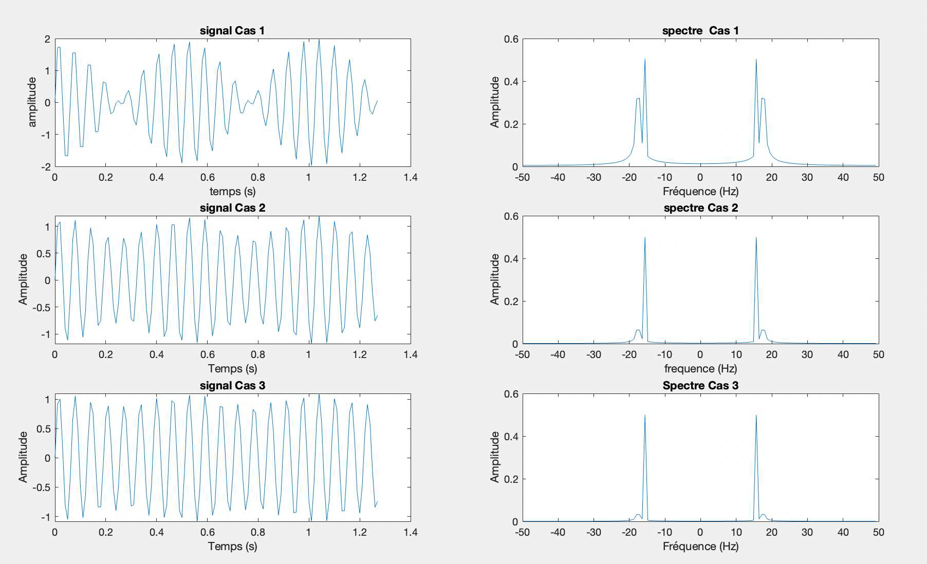
En comparant les trois cas, on peut déduire que le Cas 1 est un signal plus complexe avec des composantes de fréquence multiples, tandis que les Cas 2 et Cas 3 sont des signaux plus simples, montrant des tonalités pures avec une seule fréquence dominante. Le Cas 3 a une fréquence plus élevée que le Cas 2, ce qui signifie que le signal oscille plus rapidement dans le temps. Ces différences peuvent avoir diverses implications dans le contexte de l'analyse des signaux, telles que l'identification de la nature du signal, la détermination de la réponse d'un système, ou l'analyse harmonique pour la musique ou l'ingénierie.

# 3 c

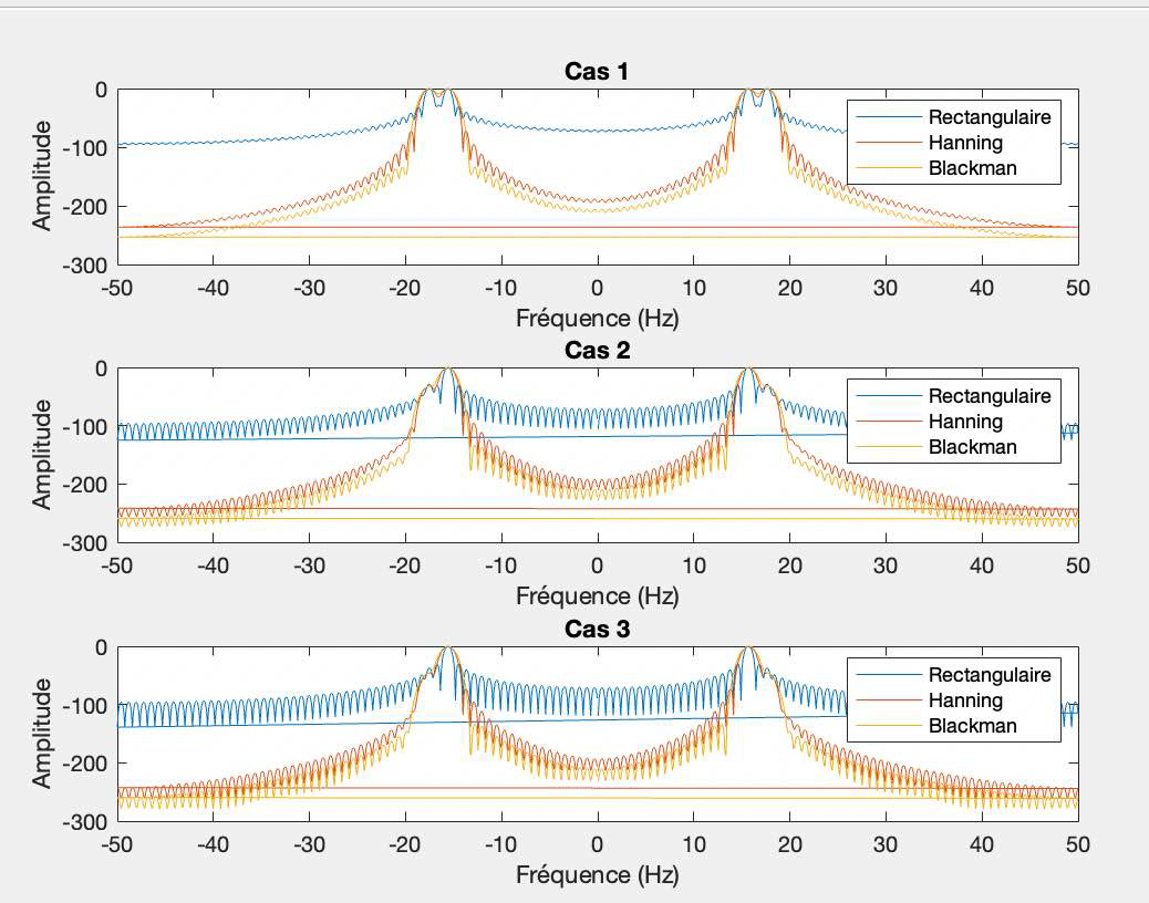
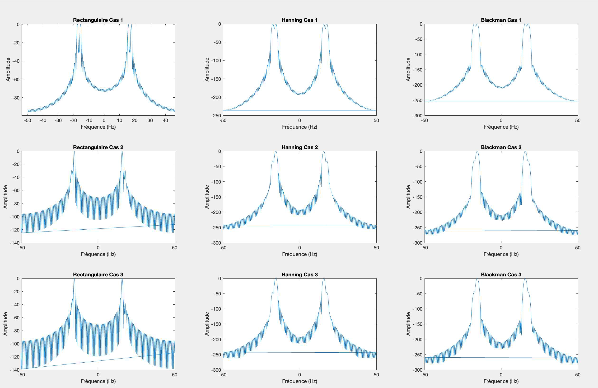
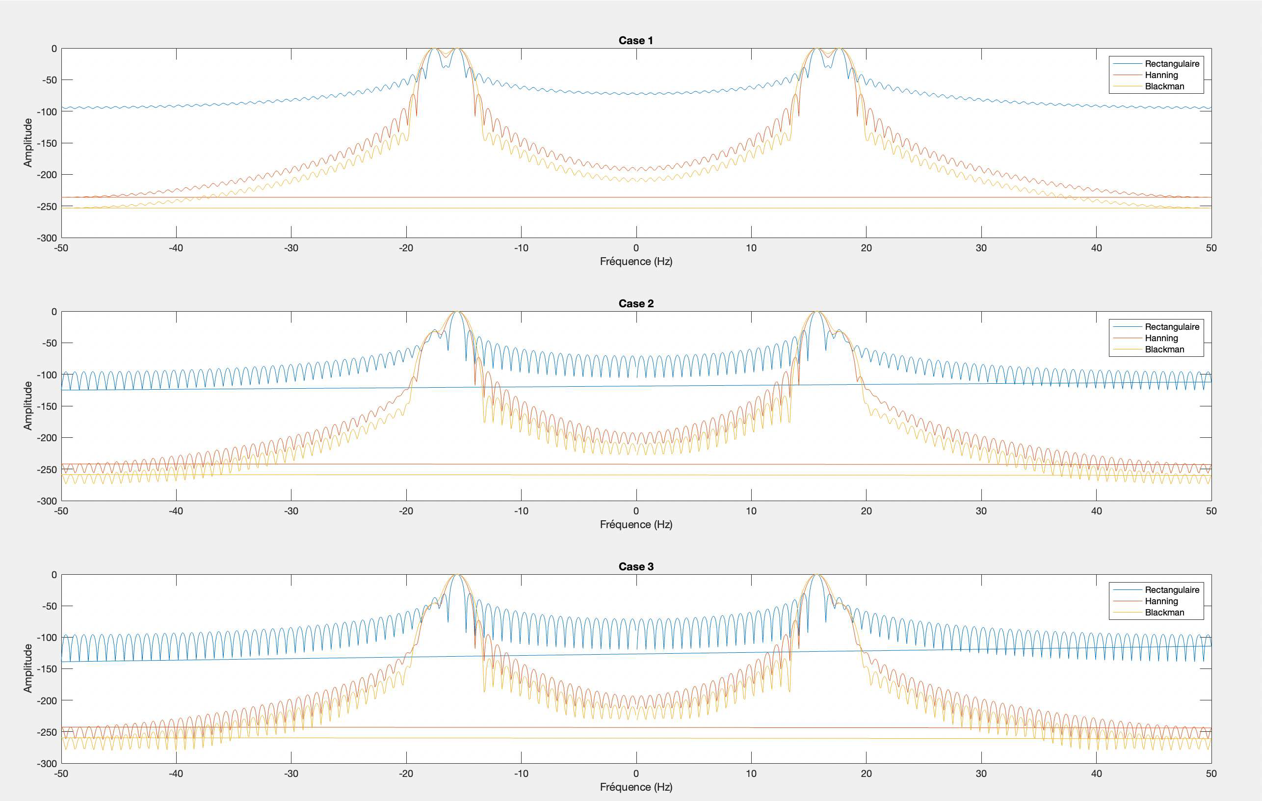
La fenêtre rectangulaire présente l'avantage d'être facile à mettre en œuvre et de ne pas altérer l'amplitude des échantillons, ce qui rend les composantes fréquentielles, plus distinguables dans ce cas précis. Cependant, elle peut poser problème si les amplitudes des composantes fréquentielles sont faibles, car elles risquent de se perdre dans les lobes, qui sont importants dans cette fenêtre. De plus, etant donné qu'elle est de largeur large, elle peut entrainer des fuites spectrals si les signaux ne sont pas representé dans la fenetre.

La fenêtre de Hanning offre une amdlioration en réduisant considérablement les lobes secondaires, ameliorant ainsi la precision spectrale. Cependant, elle conserve toujours une réponse impulsionnelle large, ce qui peut affecter la résolution temporelle. Ainsi il donne un élargissement du lobe principal, ce qui peut affecter la séparation des fréquences.

La fenêtre de Blackman, permet une meilleur réduction des lobes secondaires, ce qui est interessant pour une meilleure précision fréquentielle. Cependant, son inconvénient est qu'elle à une réponse impulsionnelle plus étroite que celle de la fenêtre de Hanning.



fe = 100;
tau = 1.28;
N = 128;
t = 0:1/fe:tau - 1/fe;

% Cas 1
f1 = 15.625; A1 = 1;
f2 = 17.578; A2 = 1;

signal1 = A1 * sin(2 * pi * f1 * t) + A2 * sin(2 * pi * f2 * t);
window1_rectangular = ones(1, N); % Fenêtre rectangulaire
window1_hanning = 0.5 * (1 - cos(2 * pi * (0:N-1) / (N-1))); % Fenêtre de Hanning
window1_blackman = 0.42 - 0.5 * cos(2 * pi * (0:N-1) / (N-1)) + 0.08 * cos(4 * pi * (0:N-1) / (N-1)); % Fenêtre de Blackman

signal1_rectangular = signal1(1:N) .* window1_rectangular;
signal1_hanning = signal1(1:N) .* window1_hanning;
signal1_blackman = signal1(1:N) .* window1_blackman;

% Normalize spectra for Case 1
spectrum1_rectangular = abs(fft(signal1_rectangular, 1024)/N);
spectrum1_rectangular = spectrum1_rectangular / max(spectrum1_rectangular);
spectrum1_hanning = abs(fft(signal1_hanning, 1024)/N);
spectrum1_hanning = spectrum1_hanning / max(spectrum1_hanning);
spectrum1_blackman = abs(fft(signal1_blackman, 1024)/N);
spectrum1_blackman = spectrum1_blackman / max(spectrum1_blackman);

% Cas 2
f1 = 15.625; A1 = 1;
f2 = 17.578; A2 = 0.2;

signal2 = A1 * sin(2 * pi * f1 * t) + A2 * sin(2 * pi * f2 * t);
window2_rectangular = ones(1, N); % Fenêtre rectangulaire
window2_hanning = 0.5 * (1 - cos(2 * pi * (0:N-1) / (N-1))); % Fenêtre de Hanning
window2_blackman = 0.42 - 0.5 * cos(2 * pi * (0:N-1) / (N-1)) + 0.08 * cos(4 * pi * (0:N-1) / (N-1)); % Fenêtre de Blackman

signal2_rectangular = signal2(1:N) .* window2_rectangular;
signal2_hanning = signal2(1:N) .* window2_hanning;
signal2_blackman = signal2(1:N) .* window2_blackman;

% Normalize spectra for Case 2
spectrum2_rectangular = abs(fft(signal2_rectangular, 1024)/N);
spectrum2_rectangular = spectrum2_rectangular / max(spectrum2_rectangular);
spectrum2_hanning = abs(fft(signal2_hanning, 1024)/N);
spectrum2_hanning = spectrum2_hanning / max(spectrum2_hanning);
spectrum2_blackman = abs(fft(signal2_blackman, 1024)/N);
spectrum2_blackman = spectrum2_blackman / max(spectrum2_blackman);

% Cas 3
f1 = 15.625; A1 = 1;
f2 = 17.578; A2 = 0.1;

signal3 = A1 * sin(2 * pi * f1 * t) + A2 * sin(2 * pi * f2 * t);
window3_rectangular = ones(1, N); %  rectangulaire
window3_hanning = 0.5 * (1 - cos(2 * pi * (0:N-1) / (N-1))); %  Hanning
window3_blackman = 0.42 - 0.5 * cos(2 * pi * (0:N-1) / (N-1)) + 0.08 * cos(4 * pi * (0:N-1) / (N-1)); % Blackman

% appliquer les fenêtres
signal3_rectangular = signal3(1:N) .* window3_rectangular;
signal3_hanning = signal3(1:N) .* window3_hanning;
signal3_blackman = signal3(1:N) .* window3_blackman;

% Normalize spectra for Case 3
spectrum3_rectangular = abs(fft(signal3_rectangular, 1024)/N);
spectrum3_rectangular = spectrum3_rectangular / max(spectrum3_rectangular);
spectrum3_hanning = abs(fft(signal3_hanning, 1024)/N);
spectrum3_hanning = spectrum3_hanning / max(spectrum3_hanning);
spectrum3_blackman = abs(fft(signal3_blackman, 1024)/N);
spectrum3_blackman = spectrum3_blackman / max(spectrum3_blackman);

% Plotting
figure;

% Case 1
subplot(3, 1, 1);
plot(frequencies1, 20.*log(fftshift(spectrum1_rectangular)));
hold on;
plot(frequencies1_hanning, 20.*log(spectrum1_hanning));
plot(frequencies1_blackman, 20.*log(spectrum1_blackman));
hold off;
title('Case 1');
xlabel('Fréquence (Hz)');
ylabel('Amplitude');
legend('Rectangulaire', 'Hanning', 'Blackman');

% Case 2
subplot(3, 1, 2);
plot(frequencies2, 20.*log(spectrum2_rectangular));
hold on;
plot(frequencies2_hanning, 20.*log(spectrum2_hanning));
plot(frequencies2_blackman, 20.*log(spectrum2_blackman));
hold off;
title('Case 2');
xlabel('Fréquence (Hz)');
ylabel('Amplitude');
legend('Rectangulaire', 'Hanning', 'Blackman');

% Case 3
subplot(3, 1, 3);
plot(frequencies3, 20.*log(spectrum3_rectangular));
hold on;
plot(frequencies3_hanning, 20.*log(spectrum3_hanning));
plot(frequencies3_blackman, 20.*log(spectrum3_blackman));
hold off;
title('Case 3');
xlabel('Fréquence (Hz)');
ylabel('Amplitude');
legend('Rectangulaire', 'Hanning', 'Blackman');

# 4. B

1. Le temps d’étude restant le même, quelle est alors la résolution en fréquence du spectre de ce signal suréchantillonné ?

Lorsque vous suréchantillonnez un signal temporel, vous ajoutez des points entre les points initiaux, ce qui augmente la densité temporelle des échantillons. Cela a des implications directes sur la résolution en fréquence du spectre du signal suréchantillonné.

La résolution en fréquence $(\Delta f)$ est inversement proportionnelle à la durée totale T du signal, selon la relation :

$[ \Delta f = \frac{1}{T} ]$

où T est la durée totale du signal. Si le temps d'étude reste le même, la durée totale du signal reste constante. Par conséquent, lorsque vous suréchantillonnez le signal, vous ajoutez plus d'échantillons dans la même durée totale, ce qui augmente la résolution en fréquence.

La résolution en fréquence améliorée $(\Delta f')$ du signal suréchantillonné peut être approximée par la relation :

$[ \Delta f' = \frac{1}{N \cdot T} ]$

où N est le facteur de suréchantillonnage, c'est-à-dire le nombre de points ajoutés entre deux points initiaux. Ainsi, en augmentant N, vous diminuez la distance entre les fréquences adjacentes dans le spectre du signal suréchantillonné, améliorant ainsi la résolution en fréquence.

En résumé, la résolution en fréquence du spectre d'un signal suréchantillonné est améliorée en raison de la densité temporelle accrue des échantillons, et cela peut être quantifié en utilisant le facteur de suréchantillonnage N dans la relation $(\Delta f' = \frac{1}{N \cdot T})$.

2. Quelle est la période du spectre ?
La période du spectre est $f_e$ car la période du signal est $\frac{1}{T_e}$ et $f_e=\frac{1}{T_e}$

3. Retrouvez le spectre du signal suréchantilloné à partir du spectre du premier signal


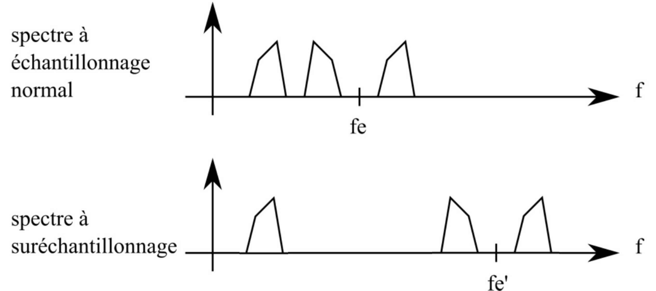
Le spectre haut est repeter à $-f_e$ et $f_e$. Donc cela s'applique également pour le signal suréchantilloné.

f1 = 50; % fréquence du sinus en Hz
fs1 = 200; % fréquence d'échantillonnage en Hz
t = (0:31) / fs1; % vecteur temps
signal1 = sin(2 * pi * f1 * t);

f2 = 500;
t2 = (0:31) / f2;
signal2 = sin(2 * pi * f1 * t2); % obtenu directement avec la fréquence

signal22 = interp1(t, signal1, t2); % obtenu a partir de s1 avec un sur échantillonnage

f3 = 1000;
t3 = (0:31) / f3;
signal3 = sin(2 * pi * f1 * t3); % obtenu directement avec la fréquence

signal33 = interp1(t, signal1, t3); % obtenu a partir de s1 avec un sur échantillonnage

% Affichage des signaux dans une seule figure avec plusieurs sous-graphiques
figure;

subplot(5,1,1);
plot(t, signal1);
title('Signal 1');

subplot(5,1,2);
plot(t2, signal2);
title('Signal 2');

subplot(5,1,3);
plot(t2, signal22);
title('Signal 22');

subplot(5,1,4);
plot(t3, signal3);
title('Signal 33');

subplot(5,1,5);
plot(t3, signal33);
title('Signal 33');