# Notes for PAZK
> [TOC]
## Abstract
- Interactive proofs(**IP**s) and arguments are cryptographic protocols that enable an untrusted prover to provide a guarantee that it performed a requested computation correctly.
- IPs allow for interaction between prover and verifier, as well as a tiny but nonzero probability that an invalid proof passes verification. Arguments(But not IPs) even permit there to be "proofs" of false statements, so long as those "proofs" require exorbitant computational power to find.
- **IP = PSPACE**
- **MIP = NEXP**
- Any argument can in principle be transformed into one that is _**zero-knowledge**_, which means that proofs reveal no information other than their own validity.
[Everything Provable is Provable in Zero-Knowledge](https://dl.acm.org/doi/pdf/10.5555/88314.88333)
- There are now no fewer than five promising approaches to designing efficient, general-purpose zero-knowledge arguments.
## Chapter 1 Introduction
- A particular goal of this survey is to describe a variety of approaches to constructing so-called zero-knowledge Succinct Non-interactive Arguments of Knowledge, or **zk-SNARKs** for short. *Succinct* means that the proofs are short. *Non-interactive* means that the proof is static, consisting of a single message from the prover. *Of Knowledge* roughly means that the protocol establishes not only that a statement is true, but also that the prover knows a **witness** to the veracity of the statement. Argument systems satisfying all of these properties have a myriad of applications throughout cryptography.
- Even though implementations of general-purpose VC protocols remain somewhat costly (especially for the prover), paying this cost can often be justified if the VC protocol is zero-knowledge, since zero-knowledge protocols enable applications that may be totally impossible without them.
- Argument systems are typically developed in a two-step process. First, an information-theoretically secure protocol, such as an **IP**, _multi-prover interactive proof_ (**MIP**), or _probabilistically checkable proof_ (**PCP**), is developed for a model involving one or more provers that are assumed to behave in some restricted manner (e.g., in an MIP, the provers are assumed not to send information to each other about the challenges they receive from the verifier). Second, the information-theoretically secure protocol is combined with cryptography to "force" a (single) prover to behave in the restricted manner, thereby yielding an argument system. This second step also often endows the resulting argument system with important properties, such as zero-knowledge, succinctness, and non-interactivity. If the resulting argument satisfies all of these properties, then it is in fact a zk-SNARK.
- Argument systems = information-theoretically secure protocol + cryptography
- information-theoretically secure protocol:
- **IP**s
- **MIP**s
- **PCP**s or _interactive oracle proofs_(**IOP**s), which is a hybrid between an IP and a PCP
- _linear_ **PCP**s
- IPs, MIPs, and PCPs/IOPs + _polynomial commitment scheme_ => succinct interactive arguments
- succinct interactive arguments + _Fiat-Shamir transformation_ => SNARK
- linear PCPs + ?(though closely related to certain polynomial commitment schemes)
- this survey covers these *cryptographic transformations* in a unified manner
- Ordering of information-theoretically secure models in this survey: IPs, MIPs, PCPs and IOPs, linear PCPs
### 1.1 Mathematical Proofs
- Informally, what we mean by a **proof** is anything that convinces someone that a statement is true
- and a **proof system** is any procedure that decides what is and is not a convincing **proof**. That is, a proof system is specified by a verification procedure that takes as input any statement and a claimed "proof" that the statement is true, and decides whether or not the proof is valid.
- __completeness__: Any true statement should have a convincing proof of its validity. 对的错不了
- __soundness__: No false statement should have a convincing proof. 错的对不了
- Ideally, the verification procedure will be __efficient__. Roughly, this means that simple statements should have short (convincing) proofs that can be checked quickly. 验证高效
- Ideally, proving should be efficient too. Roughly, this means that simple statements should have short (convincing) proofs that can be found quickly. 证明高效
- Traditionally, a __mathematical proof__ is something that can be written and checked line-by-line for correctness.
### 1.2 What kinds of non-traditional proofs will we study?
- probabilistic in nature.
- This means that the verification procedure will make **random choices**, and the soundness guarantee will hold with (very) high probability over those random choices.
- That is, there will be a (very) small probability that the verification procedure will declare a false statement to be true.
#### 1.2.1 Interactive Proofs (IPs)
- It is worth remarking on an interesting difference between IPs and traditional static proofs. Static proofs are _transferrable_, ..., In contrast, an interactive proof may not be *transferrable*.
- This is because **soundness** of the IP only holds if, every time Prover sends a response to Verifier, Prover does **not** know what challenge Verifier will respond with next. The __transcript alone__(仅凭文字记录) does not give third parties a guarantee that this holds.
#### 1.2.2 Argument Systems
- Argument systems are IPs, but where the **soundness** guarantee need only hold against cheating provers that run in *polynomial time*. Argument systems make use of cryptography. Roughly speaking, in an argument system a cheating prover cannot trick the verifier into accepting a false statement unless it breaks some cryptosystem, and breaking the cryptosystem is assumed to require *superpolynomial* time.
#### 1.2.3 Multi-Prover Interactive Proofs, Probabilistically Checkable Proofs, etc.
- MIP
- An MIP is like an IP, except that there are multiple provers, and these provers are assumed **not** to share information with each other regarding what challenges they receive from the verifier.
- PCP
- In a PCP, the proof is **static** as in a traditional mathematical proof, but the verifier is only allowed to read a small number of (possibly randomly chosen) characters from the proof.
- The PCP theorem [ALM+98, AS98] essentially states that _any_ traditional mathematical proof can be written in a format that enables this lazy reviewer to obtain a high degree of confidence in the validity of the proof by inspecting just a few words of it.
- However, by combining MIPs and PCPs with cryptography, we will see how to turn them into argument systems, and these are directly applicable in cryptographic settings. For example, we will see in **Section 9.2** how to turn a PCP into an argument system in which the prover does _not_ have to send the whole PCP to the verifier.
- Section 10.2 of this survey in fact provides a unifying abstraction, called _polynomial IOPs_, of which all of the IPs, MIPs, and PCPs that we cover are a special case. It turns out that any polynomial IOP can be transformed into an argument system with short proofs, via a cryptographic primitive called a polynomial commitment scheme.
* **polynomial IOPs** = $\{\mathsf{IPs}, \mathsf{MIPs}, \mathsf{PCPs}, \dots\}$
## Chapter 2 The Power of Randomness: Fingerprinting and Freivalds’ Algorithm
### 2.1 Reed-Solomon Fingerprinting
- Before we discuss the details of such proof systems, let us first develop an appreciation for how **randomness** can be exploited to dramatically **improve the efficiency** of certain algorithms.
#### 2.1.1 The Setting
- Alice and Bob, who trust each other and want to cooperate.
- Let us denote Alice’s file as the sequence of characters $(a_1,\dots, a_n)$, and Bob’s as $(b_1,\dots,b_n)$. Their goal is to determine whether their files are _equal_, i.e., whether $a_i = b_i$ for all $i = 1,\dots ,n$. they would like to minimize _communication_.
- A **trivial** solution: entire file and check them.
- It turns out that no _deterministic_ procedure can send less information than this trivial solution.
#### 2.1.2 The Communication Protocol
- **The High-Level Idea.**
- pick a hash function $h$ at random from family of hash functions $\mathcal{H}$
- We will think of $h(x)$ as a very short "fingerprint" of $x$.
- By **fingerprint**, we mean that $h(x)$ is a "nearly unique identifier" for $x$,
- in the sense that for any $y \neq x$, the fingerprints of $x$ and $y$ differ with high probability over the random choice of $h$, i.e.,
- for all $x \neq y, \mathsf{Pr}_{h\in \mathcal{H}}[h(x) = h(y)] \leq 0.0001$
- **The Details.**
- fix a prime number $p \geq \mathsf{max}\{m, n^2 \}$,
- For each $r \in \mathbb{F}_p$ , define $h_r(a_1, \dots, a_n) = \sum_{i = 1}^{n}a_i \cdot r^{i-1}$. The family $\mathcal{H}$ of hash functions we will consider is $\mathcal{H} = \{h_r: r \in \mathbb{F}_p\}$.
- Bob outputs **EQUAL** if $h_r(a) = h_r(b)$, and outputs **NOT-EQUAL** otherwise.
#### 2.1.3 The Analysis
- If $a_i = b_i$ for all $i = 1, \dots,n$, then Bob outputs **EQUAL** for every possible choice of $r$.
- If there is even one $i$ such that $a_i \neq b_i$, then Bob outputs **NOT-EQUAL** with probability at least $1−(n−1)/p$, which is at least $1−1/n$ by choice of $p \geq n^2$.
**Fact 2.1**. _For any two distinct (i.e., unequal) polynomials $p_a$ , $p_b$ of degree at most $n$ with coefficients in $\mathbb{F}_p$ , $p_a(x) = p_b(x)$ for at most n values of $x$ in $\mathbb{F}_p$_
#### 2.1.4 Cost of the Protocol
- send $v$ and $r$, $O(\log n)$ assuming $p \leq n^c$
#### 2.1.5 Discussion
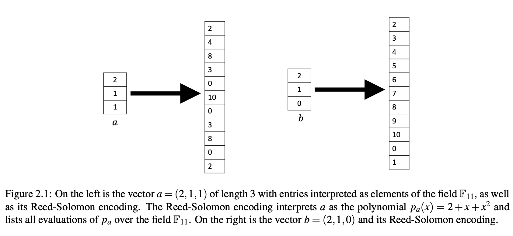
- We refer to the above protocol as Reed-Solomon fingerprinting because $p_a(r)$ in $p_a(x) = \sum_{i=1}^{n} a_i \cdot x^{i - 1}$ is actually a random entry in an _error-corrected encoding_ of the vector $(a_1, \dots, a_n)$.
- The encoding is called the **Reed-Solomon encoding**
- Reed-Solomon fingerprinting will prove particularly relevant in our study of probabilistic proof systems, owing to its algebraic structure.
- Personal idea
- why not: $p_a(x) = \sum_{i=1}^n x \cdot a_i^{i+1}$
- If there are some difference, $i \in \{x, y, z, \dots\}$ such that $a_i \neq b_i$ , then if $\sum_{i=0}^{n} a_i^{i+1} = \sum_{i=0}^{n} b_i^{i+1}$ Bob outputs **NOT-EQUAL** with probability at $0$. If $\sum_{i=0}^{n} a_i^{i+1} \neq \sum_{i=0}^{n} b_i^{i+1}$, Bob outputs **NOT-EQUAL** with probability at $1$, In this way, random numbers lose their power.
#### 2.1.6 Establishing Fact 2.1
**Fact 2.2.** _Any nonzero polynomial of degree at most $n$ over any field has at most $n$ roots._

### 2.2 Freivalds' Algorithm
- our first example of an efficient probabilistic proof system.
#### 2.2.1 The Setting
- matrices $A, B$ over $\mathbb{F}_p$, where $p > n^2$ is a prime number.
- product matrix $A \cdot B$ in time roughtly $O(n^{2.37286})$
#### 2.2.2 The Algorithm
- First,choose a random $r \in \mathbb{F}_p$,and let $x = (1, r, r^2, \dots, r^{n-1})$. Then compute $y = Cx$ and $z =A \cdot Bx$, outputting $\mathsf{YES}$ if $y = z$ and $\mathsf{NO}$ otherwise.
#### 2.2.3 Runtime
- Since multiplying an $n \times n$ matrix by an $n$-dimensional vector can be done in $O(n^2)$ time, We claim that the entire algorithm runs in time $O(n^2)$.
#### 2.2.4 Completeness and Soundness Analysis
- Letting $[n]$ denote the set $\{1,2,\dots,n\}$
- If $C = D$, then the algorithm outputs $\mathsf{YES}$ for every possible choice of $r$.
- If there is even one $(i, j) \in [n] \times [n]$ such that $C_{i,j} \neq D_{i,j}$, then Bob outputs $\mathsf{NO}$ with probability at least $1−(n−1)/p$.
#### 2.2.5 Discussion
- Whereas fingerprinting saved _communication_ compared to a deterministic protocol, Freivalds’ algorithm saves _runtime_ compared to the best known deterministic algorithm.
### 2.3 An Alternative View of Fingerprinting and Freivalds’ Algorithm
- The encoding is distance-amplifying: if a and b differ on even a single coordinate, then their encodings will differ on a $1-(n-1)/p$ fraction of coordinates.
- $p_a(x) = 2 + x + x^2 \\ p_b(x) = 2 + x$
- Personal idea:
- **distance-amplifying**,This is a kind of noise amplifier. There is only a little difference in the origin, but the image are very different. it is indeed a property of hash
- While deterministically checking equality of the two large objects would be very expensive in terms of either communication or computation time, evaluating a single entry of the each object’s encoding can be done with only logarithmic communication or in just linear time.
### 2.4 Univariate Lagrange Interpolation
- The most natural such alternative is to view $a_1,...,a_n$ as the _evaluations_ of $q_a$ over some canonical set of inputs, say, $\{0,1,...,n−1\}$.
- Indeed, as we now explain, for any list of $n$ (input, output) pairs, there is a unique univariate polynomial of degree $n − 1$ consistent with those pairs. The process of defining this polynomial $q_a$ is called __Lagrange interpolation__ for univariate polynomials.
- **Lemma 2.3** (**Univariate Lagrange Interpolation**). Let $p$ be a prime larger than $n$ and $F_p$ be the field of integers modulo $p$. For any vector $a = (a_1,\dots,a_n) \in \mathbb{F}^n$, there is a unique univariate polynomial $q_a$ of degree at most $n − 1$ such that $$q_a(i) = a_{i+1} \ \text{for} \ i = 0,\dots,n−1$$
- **Lagrange basis polynomials.** For each $i \in \{0,\dots,n−1\}$, define the following univariate polynomial $\delta_i$ over $\mathbb{F}_p$: $$\delta_i(X) = \prod_{k=0, 1, \dots, n-1: k \neq i} (X −k)/(i−k).$$
- Personal idea:
- Given a vector $a = (a_1, \dots, a_n) \in \mathbb{F}^n$, how to turn it into a polynomial?
- $p_a(X) = \sum_{i=0}^{n-1} a_{i+1} \cdot X^i$
- $q_a(X) = \sum_{j=0}^{n-1} a_{j+1} \cdot \delta_j(X)$
- $q_a(X) = \sum_{j=0}^{n-1} (a_{j+1} \cdot \prod_{k\neq j}\frac{X-k}{j-k})$
- **univariate low-degree extension**
- LDE(a):
- Given a vector $a = (a_1,\dots,a_n) \in \mathbb{F}_p^n$, the polynomial $q_a$ given in $q_a(i) = a_{i+1}$ is often called the univariate low-degree extension of $a$.
- notes::
- LDE(a), in the strictest sense, is $q_a(X) = \sum_{j=0}^{n-1} a_{j+1} \cdot \delta_j(X)$, because The highest degree is $n-1$, which is unique.
- To be more relaxed, any highest degree $O(n)$ will do, such as $2n$. With $n$ fixed points, there are many polynomials with degree $2n$.
- Loose to the minimum standard, to meet the highest order < $p$
- **Theorem 2.4.** Let $p ≥ n$ be a prime number. Given as input $a_1,\dots,a_n \in \mathbb{F}_p$, and $r \in \mathbb{F}_p$, there is an algorithm that performs $O(n)$ additions, multiplications, and inversions over $\mathbb{F}_p$, and outputs $q(r)$ for the unique univariate polynomial $q$ of degree at most $n−1$ such that $q(i) = a_{i+1}$ for $i \in \{0,1, \dots,n−1\}$.
$$\delta_i(r) = \delta_{i−1}(r)\cdot(r−(i−1))\cdot(r−i)^{−1} \cdot i^{−1} \cdot (−(n−i)).$$
## Chapter 3 Definitions and Technical Preliminaries
### 3.1 Interactive Proofs
- Given a function $f$ mapping $\{0, 1\}^n$ to a finite range $\mathcal{R}$, a $k$-message _interactive proof system_(**IP**) for $f$ consists of a probabilistic verifier algorithm $\mathcal{V}$ running in time poly($n$) and a prescribed ("honest") deterministic prover algorithm $\mathcal{P}$. Both $\mathcal{V}$ and $\mathcal{P}$ are given a common input $x \in \{0,1\}^n$, and at the start of the protocol $\mathcal{P}$ provides a value $y$ claimed to equal $f(x)$. Then $\mathcal{P}$ and $\mathcal{V}$ exchange a sequence of messages $m_1,m_2,\dots,m_k$ that are determined as follows. The IP designates one of the parties, either $\mathcal{P}$ or $\mathcal{V}$, to send the first message $m_1$. The party sending each message alternates, meaning for example that if $\mathcal{V}$ sends $m_1$, then $\mathcal{P}$ sends $m_2$, $\mathcal{V}$ sends $m_3$, $\mathcal{P}$ sends $m_4$, and so on.
- Both $\mathcal{P}$ and $\mathcal{V}$ are thought of as "next-message-computing algorithms", meaning that when it is $\mathcal{V}$'s (respectively, $\mathcal{P}$'s) turn to send a message $m_i$, $\mathcal{V}$ (respectively, $\mathcal{P}$) is run on input $(x,m_1,m_2,\dots,m_{i−1})$ to produce message $m_i$. Note that since $\mathcal{V}$ is probabilistic, any message $m_i$ sent by $\mathcal{V}$ may depend on both $(x,m1,m2,...,m_{i−1})$ and on the verifier’s internal randomness.
- The entire sequence of $k$ messages $t := (m_1,m_2,\dots,m_k)$ exchanged by $\mathcal{P}$ and $\mathcal{V}$, along with the claimed answer $y$, is called a **transcript**. At the end of the protocol, $\mathcal{V}$ must output either $0$ or $1$, with $1$ indicating that the verifier accepts the prover’s claim that $y = f(x)$ and $0$ indicating that the verifier rejects the claim. The value output by the verifier at the end of the protocol may depend on both the transcript $t$ and the verifier’s internal randomness.
- Denote by $\text{out}(\mathcal{V},x,r,\mathcal{P}) \in \{0,1\}$ the output of verifier $\mathcal{V}$ on input $x$ when interacting with deterministic prover strategy $\mathcal{P}$, with $\mathcal{V}$'s internal randomness equal to $r$. For any fixed value $r$ of $\mathcal{V}$'s internal randomness, $\text{out}(\mathcal{V},x,r,\mathcal{P})$ is a deterministic function of $x$ (as we have restricted our attention to deterministic prover strategies $\mathcal{P}$).
- **Definition 3.1.** An interactive proof system $(\mathcal{V}, \mathcal{P})$ is said to have completeness error $\delta_c$ and soundness error $\delta_s$ if the following two properties hold.
- 1. (_Completeness_) For every $x \in \{0,1\}^n$, $\text{Pr}_r[\text{out}(\mathcal{V},x,r,\mathcal{P}) = 1] \geq 1− \delta_c.$
- 2. (_Soundness_) For every $x \in \{0,1\}^n$ and _every_ deterministic prover strategy $\mathcal{P}^\prime$, if $\mathcal{P}^\prime$ sends a value $y \neq f(x)$ at the start of the protocol, then $\text{Pr}_r[\text{out}(\mathcal{V},x,r,\mathcal{P^\prime}) = 1] \leq \delta_s.$
- An interactive proof system is valid if $\delta_c,\delta_s ≤ 1/3$.
- The two costs of paramount importance in any interactive proof are $\mathcal{P}$'s runtime and $\mathcal{V}$’s runtime, but there are other important costs as well: $\mathcal{P}$'s and $\mathcal{V}$'s space usage, the total number of bits communicated, and the total number of messages exchanged. If $\mathcal{V}$ and $\mathcal{P}$ exchange $k$ messages, then $⌈k/2⌉$ is referred to as the round complexity of the interactive proof system. The round complexity is the number of “back-and-forths” in the interaction between $\mathcal{P}$ and $\mathcal{V}$. If $k$ is odd, then the final “back-and-forth” in the interaction is really just a “back” with no “forth”, i.e., it consists of only one message from prover to verifier.
- Interactive proofs were introduced in 1985 by Goldwasser, Micali, and Rackoff [GMR89] and Babai [Bab85].
### 3.2 Argument Systems
- **Definition 3.2.** An argument system for a function $f$ is an interactive proof for $f$ in which the soundness condition is only required to hold against prover strategies that run in polynomial time.
- Definition 3.2. is _computational soundness_
- Definition 3.1. is _statistical soundness or information-theoretic soundness_
- Argument systems aka _computationally sound proofs_
- The use of **cryptography** often allows argument systems to achieve additional desirable properties that are unattainable for interactive proofs, such as **reusability** (i.e., the ability for the verifier to reuse the same "secret state" to outsource many computations on the same input), public **verifiability**, etc.
### 3.3 Robustness of Definitions and the Power of Interaction
- (Perfect vs. Imperfect Completeness)
- all of the interactive proofs that we will see in this manuscript actually satisfy *perfect completeness*, meaning that $\delta_c = 0$. That is, the honest prover in our IPs and arguments will always convince the verifier that it is honest.
- It is actually known [FGM+89] that any IP for a function $f$ with $\delta_c ≤ \frac{1}{3}$ can be transformed into an IP for $f$ with **perfect completeness**, with a polynomial blowup in the verifier’s costs
- (Soundness Error)
- In all of the interactive proofs that we see in this survey, the soundness error will always be proportional to $1/|\mathbb{F}|$, where $\mathbb{F}$ is the field over which the interactive proof is defined.
- A cheating prover successfully tricking a verifier to accept a false claim can have *catastrophic* effects in cryptographic applications.
- Soundness error of any IP or argument can also be generically reduced from $\delta_s$ to $\delta_s^k$ by repeating the protocol $\Theta(k)$ times in sequence and rejecting unless the verifier accepts in a majority of the repetitions.
- (Public vs. Private Randomness)
- _private randomness_
- One can also consider IPs in which the verifier’s randomness is public—that is, any coin tossed by $\mathcal{V}$ is made visible to the prover as soon as it is tossed. We will see that such **public-coin** IPs are particularly useful, because they can be combined with cryptography to obtain argument systems with important properties (see Chapter 5 on the Fiat-Shamir transformation).
- Public coin is the prerequisite for applying Fiat-Shamir transformation
- We will not need to utilize such transformations in this manuscript because all of the IPs that we give are naturally **public coin** protocols.
- (Deterministic vs. Probabilistic Provers)
- In this manuscript, the honest prover in all of our IPs and ar- guments will naturally be deterministic, so we will have no need to exploit this generic transformation from randomized to deterministic prover strategies.
- **Interactive Proofs for Languages Versus Functions.**
- The previous descriptions are all about IP for function $f$,
- We need to define the language and then define the IP for language
- We can associate any decision problem $f$ with the subset $\mathcal{L} \subseteq \{0, 1\}^n$ consisting of "yes-instance**s**" for $f$. Any subset $\mathcal{L} \subseteq \{0, 1\}^n$ is called a ***language***.
- The formalization of IPs for languages differs slightly from that for functions (Definition 3.1). We briefly describe this difference because celebrated results in complexity theory regarding the power of IPs and their variants (e.g., **IP = PSPACE** and **MIP = NEXP**) refer to IPs for languages.
- Language's **Soundness**. For any $x \notin \mathcal{L}$, then for every prover strategy, the verifier rejects with high probability.
- Function's **Soundness**. For every $x \in \{0,1\}^n$ and _every_ deterministic prover strategy $\mathcal{P}^\prime$, if $\mathcal{P}^\prime$ sends a value $y \neq f(x)$ at the start of the protocol, then $\text{Pr}_r[\text{out}(\mathcal{V},x,r,\mathcal{P^\prime}) = 1] \leq \delta_s.$
- **NP and IP.**
- Let **IP** be the class of all languages solvable by an interactive proof system with a polynomial time verifier. The class **IP** can be viewed as an interactive, randomized variant of the classical complexity class **NP** (**NP** is the class obtained from **IP** by restricting the proof system to be non-interactive and deterministic, meaning that the completeness and soundness errors are $0$).
- **By Your Powers Combined, I am IP.**
- The key to the power of interactive proofs is the __combination__ of randomness and interaction.
### 3.4 Schwartz-Zippel Lemma
- degree of multivariate polynomial:
- the degree of a term of $g$ is the sum of the exponents of the variables in the term.
- The total degree of $g$ is the maximum of the degree of any term of $g$
- **Lemma 3.3** (**Schwartz-Zippel Lemma**). Let $\mathbb{F}$ be any field, and let $g: \mathbb{F}^m \rightarrow \mathbb{F}$ be a nonzero $m$-variate polynomial of total degree at most $d$. Then on any finite set $S \subseteq \mathbb{F}$, $$\text{Pr}_{x\leftarrow S^m}[g(x) = 0] \leq d/|S|.$$
- Here, $x\leftarrow S^m$ denotes an $x$ drawn **uniformly at random** from the product set $S^m$, and $|S|$ denotes the size of $S$. In words, if $x$ is chosen uniformly at random from $S^m$, then the probability that $g(x) = 0$ is at most $d/|S|$. In particular, any two distinct polynomials of total degree at most d can agree on at most a $d/|S|$ fraction of points in $S^m$.
### 3.5 Low Degree and Multilinear Extensions
- **Motivation and comparison to univariate Lagrange interpolation.**
- In this section, we consider multivariate functions $f$, more specifically defined over the $v$-variate domain $\{0,1\}^v$. Note that when $v = \log n$, the domain $\{0,1\}^v$ has the same size as the univariate domain $\{0,1,...,n−1\}$.
- Specifically, any function $f$ mapping $\{0, 1\}^v \rightarrow \mathbb{F}$ has an extension polynomial that is multilinear, meaning it has degree at most $1$ in each variable. This implies that the total degree of the polynomial is at most $v$, which is logarithmic in the domain size $2^v$.
- Multivariate polynomials with ultra-low degree in each variable turn out to be especially useful when designing interactive proofs with **small communication and fast verification**.
- **Details of polynomial extensions for multivariate functions.**
- Let $\mathbb{F}$ be any finite field, and let $f: \{0, 1\}^v \rightarrow \mathbb{F}$ be any function mapping the $v$-dimensional Boolean hypercube to $\mathbb{F}$. A $v$-variate polynomial $g$ over $\mathbb{F}$ is said to be an __extension__ of $f$ if $g$ agrees with f at all Boolean-valued inputs, i.e., $g(x) = f(x)$ for all $x \in \{0, 1\}^v$. Here, the domain of the $v$-variate polynomial $g$ over $F$ is $\mathbb{F}^v$, and $0$ and $1$ are respectively associated with the additive and multiplicative identity elements of $\mathbb{F}$.
- a distance-amplifying encoding of $f$
- **Definition 3.4.** A multivariate polynomial $g$ is multilinear if the degree of the polynomial in each variable is at most one.
- For example, the polynomial $g(x_1,x_2) = x_1x_2 +4x_1 +3x_2$ is multilinear, but the polynomial $h(x_1,x_2) = x_2^2 + 4x_1 + 3x_2$ is not. Throughout this survey, we will frequently use the following fact.
- **Fact 3.5.** Any function $f: \{0, 1\}^v \rightarrow \mathbb{F}$ has a unique multilinear extension (**MLE**) over $\mathbb{F}$, and we reserve the notation $\widetilde{f}$ for this special extension of $f$
- **Lemma 3.6** (**Lagrange interpolation of multilinear polynomials**). Let $f: \{0, 1\}^v \rightarrow \mathbb{F}$ be any function. Then the following multilinear polynomial $\widetilde{f}$ extends $f$: $$\widetilde{f}(x_1,\dots,x_v) = \sum_{w\in \{0, 1\}^v} f(w)\cdot \chi_w(x_1,\dots,x_v),$$ where, for any $w = (w_1,\dots,w_v)$, $$\chi_w(x_1, \dots, x_v) := \prod_{i=1}^v (x_iw_i + (1-x_i)(1-w_i)).$$ The set $\{\chi_w: w \in \{0,1\}^v\}$ is referred to as the set of multilinear Lagrange basis polynomials with interpolating set $\{0,1\}^v$.
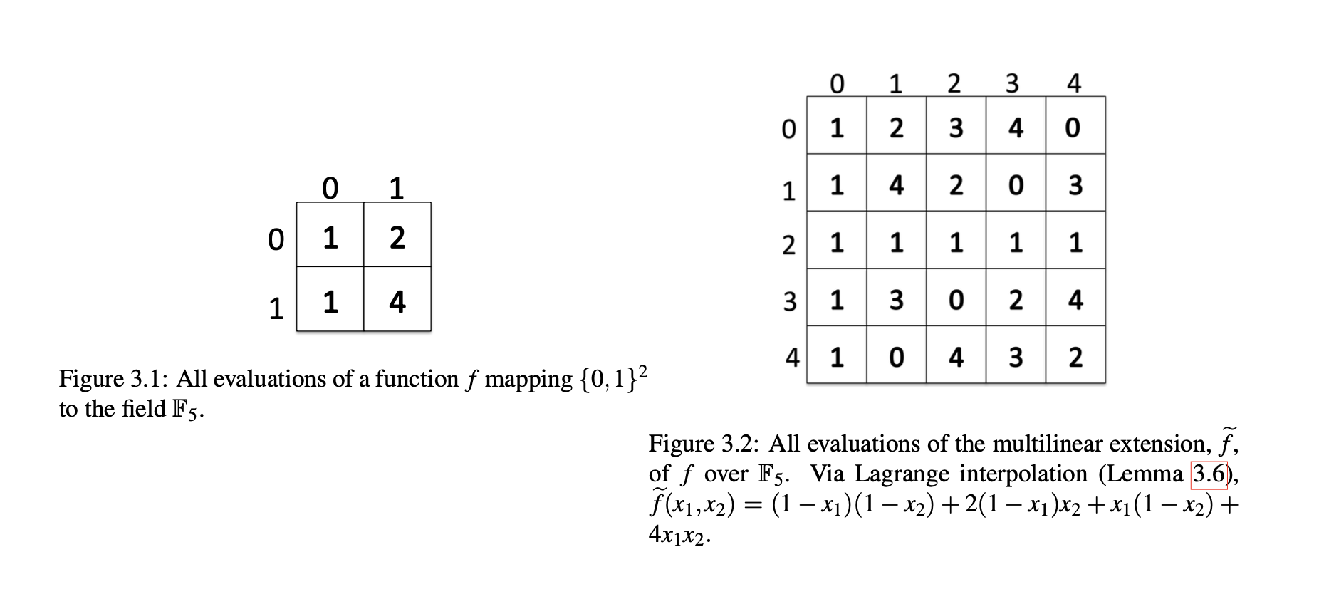
$$f(0, 0) = 1 \quad f(0,1) = 2 \quad f(1,0) = 1 \quad f(1,1) = 4$$
$$\begin{align*}\chi_{(0,0)}(x_1, x_2) &= (1-x_1)(1-x_2) \\ \chi_{(0,1)}(x_1, x_2) &= (1-x_1)x_2 \\ \chi_{(1,0)}(x_1, x_2) &= x_1(1-x_2) \\ \chi_{(1,1)}(x_1, x_2) &= x_1x_2 \end{align*}$$
$$\begin{align*} \widetilde{f}(x_1, x_2) &= \sum_{w\in \{0,1\}^2} f(w) \cdot \chi_w(x_1, x_2) \\ &= (1-x_1)(1-x_2) + 2(1-x_1)x_2 + x_1(1-x_2) + 4x_1x_2 \\ &= 1-x_1 -x_2 + x_1x_2 + 2x_2 -2x_1x_2 + x_1 - x_1x_2 + 4x_1x_2 \\ &=2x_1x_2 + x_2 + 1 \end{align*}$$
- **Algorithms for evaluating the multilinear extension of $f$.**
- [CTY11]: $O(n\log n)$ time and $O(\log n)$ space
- [VSBW13]: $O(n)$ time and $O(n)$ space
## Chapter 4 Interactive Proofs
The first interactive proof that we cover is the sum-check protocol
### 4.1 The Sum-Check Protocol
- Suppose we are given a $v$-variate polynomial $g$ defined over a finite field $\mathbb{F}$. The purpose of the sum-check protocol is for prover to provide the verifier with the following sum: $$H:=\sum_{b_1 \in \{0, 1\}} \sum_{b_2 \in \{0,1\}} \cdots \sum_{b_v \in \{0,1\}} g(b_1, \dots, b_v). \quad (4.1)$$
- **Remark 4.1.** In full generality, the sum-check protocol can compute the sum $\sum_{b \in B^v} g(b)$ for any $B \subseteq \mathbb{F}$, but most of the applications covered in this survey will only require $B = \{0, 1\}$.
- Description of **Sum-Check Protocol**.
- At the start of the protocol, the prover sends a value $C_1$ claimed to equal the value $H$ defined in Equation (4.1).
- In the first round, $\mathcal{P}$ sends the univariate polynomial $g_1(X_1)$ claimed to equal $$\sum_{(x_2, \dots, x_v) \in \{0, 1\}^{v-1}} g(X_1, x_2, \dots, x_v).$$ $\mathcal{V}$ checks that $$C_1 = g_1(0) + g_1(1),$$ and that $g_1$ is a univariate polynomial of degree at most $\text{deg}_1(g)$, rejecting if not. Here, $\text{deg}_j(g)$ denotes the degree of $g(X_1, \dots, X_v)$ in variable $X_j$.
- $\mathcal{V}$ chooses a random element $r_1 \in \mathbb{F}$, and sends $r_1$ to $\mathcal{P}$.
- In the $j$th round, for $1 < j < v$, $\mathcal{P}$ sends to $\mathcal{V}$ a univariate polynomial $g_j(X_j)$ claimed to equal $$\sum_{(x_{j+1}, \dots, x_v)\in \{0,1\}^{v-j}} g(r_1,\dots, r_{j-1},X_j,x_{j+1}, \dots, x_v).$$ $\mathcal{V}$ checks that $g_j$ is a univariate polynomial of degree at most $\text{deg}_j(g)$, and that $g_{j-1}(r_{j-1}) = g_j(0) + g_j(1)$, rejecting if not.
- $\mathcal{V}$ chooses a random element $r_j \in \mathbb{F}$, and send $r_j$ to $\mathcal{P}$.
- In Round $v$, $\mathcal{P}$ sends to $\mathcal{V}$ a univariate polynomial $g_v(X_v)$ claimed to equal $$g(r_1, \dots, r_{v-1}, X_v).$$ $\mathcal{V}$ checks that $g_v$ is a univariate polynomial of degree at most $\text{deg}_v(g)$, rejecting if not and also checks that $g_{v-1}(r_{v-1}) = g_v(0) + g_v(1)$.
- $\mathcal{V}$ chooses a random element $r_v \in \mathbb{F}$ and evaluates $g(r_1, \dots, r_v)$ with a single oracle query to $g$ . $\mathcal{V}$ checks that $g_v(r_v) = g(r_1, \dots, r_v)$, rejecting if not.
- if $\mathcal{V}$ has not yet rejected, $\mathcal{V}$ halts and accepts.
- **Example Execution of the Sum-Check Protocol.**
Let $g(X_1,X_2,X_3) = 2X_1^3 + X_1X_3 + X_2X_3.$
- At the start of the protocol, $\mathcal{P}$ sends $$\begin{align*}C_1 &= g(0,0,0) + g(0,0,1) + g(0,1,0) + g(0,1,1) + g(1,0,0) + g(1,0,1) + g(1,1,0) + g(1,1,1) \\ &= 0 + 0 + 0 + 1 + 2 + (2+1) + 2 + (2+1+1) \\ &= 12 \end{align*}$$ to $\mathcal{V}$.
- **Round 1**: $\mathcal{P}$ sends the univariate polynomial $g_1(X_1)$ equal to: $$\begin{align*} g_1(X_1) &= g(X_1, 0, 0) + g(X_1, 0, 1) + g(X_1, 1, 0) + g(X_1, 1, 1) \\ &= 2X_1^3 + (2X_1^3 + X_1) + 2X_1^3 + (2X_1^3 + X_1X_3 + X_2X_3) \\ &= 8X_1^3 + 2X_1 + 1 \end{align*}$$ $\mathcal{V}$ checks $$\begin{align*}g_1(0) + g_1(1) &= 1 + (8 + 2 + 1) \\ &= 12\\ &= C_1\end{align*}$$ and $g_1(X_1)$'s degree is at most $\text{deg}_1(g)$.
- $\mathcal{V}$ chooses a random element $r_1 = 7$ and sneds it to $\mathcal{P}$.
- **Round 2**: $\mathcal{P}$ sends to $\mathcal{V}$ a univariate polynomial $g_2(X_2)$ equal to: $$\begin{align*} g_2(X_2) &= g(7, X_2, 0) + g(7, X_2, 1) \\ &= 686 + (686 + 7 + X_2) \\ &= X_2 + 1379\end{align*}$$ $\mathcal{V}$ checks that $$\begin{align*}g_1(r_1) &= g_1(7) \\ &= 8\cdot 7^3 + 2\cdot 7 + 1 \\ &= 2759 \\ g_2(0) + g_2(1) &= 1379 + (1379+1) \\ &= 2759 \\ &= g_1(r_1)\end{align*}$$ and $g_2$ is a univariate polynomial of degree at most $\text{deg}_2(g)$.
- $\mathcal{V}$ chooses a random element $r_2 = 13$, and send $r_2$ to $\mathcal{P}$.
- **Round 3**, $\mathcal{P}$ sends to $\mathcal{V}$ a univariate polynomial $g_3(X_3)$ claimed to equal $$g_3(X_3) = g(7, 13, X_3)= 686 + 20X_3.$$ $\mathcal{V}$ checks that $g_3$ is a univariate polynomial of degree at most $\text{deg}_3(g)$, and also checks that $$\begin{align*}g_2(r_2) &= 13 + 1379 \\ &= 1392 \\ g_3(0) + g_3(1) &= 686 + (686 + 20) \\ &= 1392 \\ &= g_2(r_2)\end{align*}$$.
- $\mathcal{V}$ chooses a random element $r_3 = 19$ and evaluates $$\begin{align*}g(r_1, r_2, r_3) &= 2r_1^3 + r_1r_3 + r_2r_3 \\ &= 2\cdot 7^3 + 7\cdot19 + 13\cdot19 \\ &=1066 \\ g_3(r_3) &= 686 + 20r_3 \\ &= 686 + 20 \cdot 19 \\ &= 1066 \\ &= g(r_1, r_2, r_3) \end{align*} $$ with a single oracle query to $g$ . $\mathcal{V}$ checks that $g_3(r_3) = g(r_1, \dots, r_v)$
- if $\mathcal{V}$ has not yet rejected, $\mathcal{V}$ halts and accepts.
- **Completeness and Soundness.**
- **Proposition 4.1.** Let $g$ be a $v$-variate polynomial of degree at most $d$ in each variable, defined over a finite field $\mathbb{F}$. For any specified $H \in \mathbb{F}$, let $\mathcal{L}$ be the language of polynomials $g$ (given as an oracle) such that $$H = \sum_{b_1 \in \{0, 1\}} \sum_{b_2 \in \{0,1\}} \cdots \sum_{b_v \in \{0, 1\}} g(b_1,\dots,b_v).$$ The sum-check protocol is an interactive proof system for $\mathcal{L}$ with completeness error $\delta_c = 0$ and soundness error $\delta_s \leq vd/|\mathbb{F}|.$
- **Preview: Why multilinear extensions are useful: ensuring a fast prover.** We will see several scenarios where it is useful to compute $H=\sum_{x\in \{0,1\}^v} f(x)$ for some function $f: \{0,1\}^v \rightarrow \mathbb{F}$ derived from the verifier’s input. We can compute $H$ by applying the sum-check protocol to any low-degree extension $g$ of $f$. When $g$ is itself a product of a small number of multilinear polynomials, then the prover in the sum-check protocol applied to $g$ can be implemented extremely efficiently. Specifically, as we show later in Lemma 4.5, Lemma 3.6 (which gave an explicit expression for $\widetilde{f}$ in terms of Lagrange basis polynomials) can be exploited to ensure that enormous cancellations occur in the computation of the prover’s messages, allowing fast computation.
- **Preview: Why using multilinear extensions is not always possible: ensuring a fast verifier.** Although the use of the **MLE** $\widetilde{f}$ typically ensures fast computation for the prover, $\widetilde{f}$ cannot be used in all applications. The reason is that the verifier has to be able to evaluate $\widetilde{f}$ at a random point $r \in \mathbb{F}^v$ to perform the final check in the sum-check protocol, and in some settings, this computation would be too costly.
### 4.2 First Application of Sum-Check: #SAT ∈ IP
### 4.4 Third Application: Super-Efficient IP for MATMULT
- Matrix Multiplication($\text{M}\small{\text{AT}}\normalsize{\text{M}}\small{\text{ULT}}$)
- $C = A \cdot B$
#### The Protocol
Given $n \times n$ input matrix $A, B$, recall that we denote the product matrix $A \cdot B$ by $C$. And as in Section 4.3, we interpret $A$, $B$, and $C$ as functions $f_A$, $f_B$, $f_C$ mapping $\{0,1\}^{\log n} \times \{0,1\}^{\log n}$ to $\mathbb{F}$ via: $$f_A(i_1,\dots,i_{\log n}, j_1,\dots, j_{\log n}) = A_{ij}.$$ As usual, $\widetilde{f_A}$, $\widetilde{f_B}$, and $\widetilde{f}_C$ denote the MLEs of $f_A$, $f_B$, and $f_C$.
$\quad$ It is cleanest to describe the protocol for $\text{M}\small{\text{AT}}\normalsize{\text{M}}\small{\text{ULT}}$ as a protocol for evaluating $\widetilde{f_C}$ at any given point $(r_1,r_2) \in \mathbb{F}^{\log n \times \log n}$. As we explain later (see Section 4.5), this turns out to be sufficient for application problems such as graph diameter and triangle counting.
$\quad$ The protocol for computing $\widetilde{f_C}(r_1,r_2)$ exploits the following explicit representation of the polynomial $\widetilde{f_C}(x,y)$.
### 4.6 The GKR Protocol and Its Efficient Implementation
#### 4.6.1 Motivation
- We need IP protocols that solve prover-friendly problems.
- Can't the verifier just ignore the prover and solve the problem without help? One answer is that this section will describe protocols in which the verifier runs **much faster** than would be possible without a prover. Specifically, $\mathcal{V}$ will run linear time, doing little more than **just reading the input**.
#### 4.6.4 Protocol Details
- **Notation.** Suppose we are given a layered arithmetic circuit $\mathcal{C}$ of size $S$, depth $d$, and fan-in two ($\mathcal{C}$ may have more than one output gate). Number the layers from $0$ to $d$, with $0$ being the output layer and $d$ being the input layer. Let $S_i$ denote the number of gates at layer $i$ of the circuit $\mathcal{C}$. Assume $S_i$ is a power of $2$ and let $S_i = 2^{k_i}$. The GKR protocol makes use of several functions, each of which encodes certain information about the circuit.
- if only $1$ output gate: $S =\sum_{i = 0}^{d-1} S_i = 2^d - 1$
- fan-in two: every gate have $2$ input
- Number the gates at layer $i$ from $0$ to $S_i − 1$, and let $W_i: \{0, 1\}^{k_i} \rightarrow \mathbb{F}$ denote the function that takes as input a binary gate label, and outputs the corresponding gate’s value at layer $i$. As usual, let $\widetilde{W}_i$ denote the multilinear extension of $W_i$. See Figure 4.12, which depicts an example circuit $\mathcal{C}$ and input to $\mathcal{C}$ and describes the resulting function $W_i$ for each layer $i$ of $\mathcal{C}$.
- the **GKR** protocol also makes use of the notion of a "wiring predicate"(plonk wire contraint?) that encodes which pairs of wires from layer $i + 1$ are connected to a given gate at layer $i$ in $\mathcal{C}$. Let $\text{in}_{1, i}, \text{in}_{2,i}: \{0, 1\}^{k_i} \rightarrow \{0, 1\}^{k_{i+1}}$ **denote** the functions that take as input the of the first and second in-neighbor of gate $a$, So, for example, if gate $a$ at layer $i$ computes the sum of gates $b$ and $c$ at layer $i+1$, then $\text{in}_{1, i}(a) = b$ and $\text{in}_{2, i}(a) = c$.
-
## Chapter 5 Publicly Verifiable, Non-interactive Arguments via Fiat-Shamir
### 5.2 The Fiat-Shamir Transformation
- **Avoiding a common vulnerability.** For the Fiat-Shamir transformation to be secure in settings where an adversary can choose the input $x$ to the IP or argument, it is essential that $x$ be appended to the list that is hashed in each round. This property of soundness against adversaries that can choose $x$ is called **adaptive soundness**. Some real-world implementations of the Fiat-Shamir transformation have missed this detail, leading to attacks [BPW12, HLPT20]. In fact, this precise error was recently identified in several popular SNARK deployments, leading to critical vulnerabilities. Sometimes, the version of Fiat-Shamir that includes $x$ in the hashing is called **strong Fiat-Shamir**, while the version that omits it is called **weak Fiat-Shamir**.
- Here is a sketch of the attack if the adversary can choose $x$ and $x$ is not hashed within the Fiat-Shamir transformation. For concreteness, consider a prover applying the GKR protocol to establish that $\mathcal{C}(x) = y$. In the GKR protocol, the verifier $\mathcal{V}$ completely ignores the input $x \in \mathbb{F}^n$ until the final check in the protocol, when $\mathcal{V}$ checks that the multilinear extension $\widetilde{x} of $x$ evaluated at some randomly chosen point $r$ equals some value $c$ derived from previous rounds. The adversary can easily generate a transcript for the Fiat-Shamir-ed protocol that passes all of the verifier’s checks except the final one. To pass the final check, the adversary can choose any input $x \in \mathbb{F}^n$ such that $\widetilde{x}(r) = c$ (such an input $\widetilde{x}$ can be identified in linear time). The transcript convinces the verifier of the Fiat-Shamir-ed protocol to accept the claim that $\mathcal{C}(x) = y$. Yet there is no guarantee that $\mathcal{C}(x) = y$, as $x$ may be an arbitrary input satisfying $\widetilde{x}(r) = c$. See Exercise 5.2, which asks the reader to work through the details of this attack.
Note that in this attack, the prover does not necessarily have "perfect control" over the inputs $x$ for which it is able to produce convincing $proofs$ that $\mathcal{C}(x) = y$. This is because $x$ is constrained to satisfy $\widetilde{x}(r) = c$ for some values $r$ and $c$ that depend on the random oracle. This may render the attack somewhat benign in some applications. Nonetheless, practitioners should take care to avoid this vulnerability, especially since including $x$ in the hashing is rarely a significant cost in practice.
## Chapter 6 Front Ends: Turning Computer Programs Into Circuits
### 6.1 Introduction
- Rather, they typically have a computer program written in a high-level programming language like Java or Python, and want to execute the program on their data. In order for the GKR protocol to be useful in this setting, we need an efficient way to turn high-level computer programs into arithmetic circuits. We can then apply the GKR protocol (or any other interactive proof or argument system for circuit evaluation) to the resulting arithmetic circuit.
- Most general purpose argument system implementations work in this two-step manner. First, a computer program is compiled into a model amenable to probabilistic checking, such as an arithmetic circuit or arithmetic circuit satisfiability instance. Second, an interactive proof or argument system is applied to check that the prover correctly evaluated the circuit. In these implementations, the program-to-circuit compiler is referred to as the front end and the argument system used to check correct evaluation of the circuit is called the back end.
- a computer program to an arithmetic circuit or arithmetic circuit satisfiability instance
- an interactive proof or argument system to check that the prover correctly evaluated in the circuit
> [Proofs, Arguments, and Zero-Knowledge](https://people.cs.georgetown.edu/jthaler/ProofsArgsAndZK.html)
 Sign in with Wallet


