Recommendation Systems Report

The definitions presented in this report are a compilation and reinterpretation sourced from various references, each attributed in my best capacity. It is important to clarify that I did not develop nor contribute to the creation of any of the algorithms discussed. Rather, I have packaged them into a standardized interface for the purpose of testing and exploring different recommendation systems with modifications to suit the testing and implementation frameworks.

All code available and used to create this report can be found at this [repository](https://github.com/NeneWang/recommendation-systems-exploration).

The final processed data used to train and test the models are derived from their original source described below. [Data found at data.zip](https://github.com/NeneWang/recommendation-systems-exploration/blob/master/data/v3_recommender_datasets.zip).

## Project Description

Recommendation Engine Research for Product Recommendations: This project involves developing a Jupyter Notebook to experiment with and evaluate various recommendation
algorithms:

While the initial objectives were the algorithms above. In the end I ended using different algorithms derived from above. And some algorithms such as `knn` were also used instead for parameters optimization instead.

Turns out also that `knn` is a subset of `collaborative filtering` algorithms
https://surprise.readthedocs.io/en/stable/knn_inspired.html#surprise.prediction_algorithms.knns.KNNBasic

The performance of these models will be assessed through a split of the dataset into training and testing subsets, The AI will be tested by providing an incomplete transaction historial of the user. And the model will be graded given the recommendation output produced from such historial if it matches any of the missing transactions.

The project culminates in designing an interactive application that leverages user transaction history to predict recommendations

## Data

### Original Datasets

| Dataset | Author | Link |
|--|--|--|
Steam Games | Anton Kozyriev (Steam) | https://www.kaggle.com/datasets/antonkozyriev/game-recommendations-on-steam?select=games.csv
| The Movies Dataset | MovieLens | https://www.kaggle.com/datasets/rounakbanik/the-movies-dataset
| Book Recommendation Dataset | MÖBIUS | https://www.kaggle.com/datasets/arashnic/book-recommendation-dataset

### Standarized Recommendable Schema

The expected standarized products dataset:

**Products**

| name | type | description |
| -------------- | ---- | ----------------------------------------- |
| id | str | Unique identifier of the product |
| product_title | str | Title of the product |
| product_image | str | Image of the product |
| product_price | int | Price of the product (if available) |
| product_soup | str | All Aggregated Description of the product |
| product_tags | str | List of tags of the product, sep by comma |

**Transactions**

| name | type | description |
| ---------- | ---- | ------------------------------------ |
| id | str | Unique identifier of the transaction |
| user_id | str | Unique identifier of the user |
| product_id | str | Unique identifier of the product |
| rate | int | Positive association rating |

**Users**

| name | type | description |
| ------------ | ---- | ----------------------------- |
| id | str | Unique identifier of the user |
| age | int | Age of |
| details_soup | str | All Aggregated Description of |

### All Datasets

For data Clean up, I had different strategies for cleaning up data Versions V1, V2, V3


### V1 Cleanup streategy
V1 ensured that all transactions reflected would have at least treshhold amount of books and users repeated.

Objective
- Standarize Data into common schema across platforms
- Iteratively Remove transactions containing irrelevant product and users

The Datasets from different sources were mapped into the common Standarized Datasets Schema described at [Standarized Recommendable Schema](#Standarized-Recommendable-Schema)

Iteratively runs remove unde interactions whereas the product and

while(prev_transaction_count != len(transactions)):
    transactions = remove_under_interactions(transactions, "product_id", product_treshold)
    transactions = remove_under_interactions(transactions, "user_id", user_treshhold)
    prev_transaction_count = len(transactions)

### V2 Cleanup Strategy

- Cleanup Code: https://github.com/NeneWang/recommendation-systems-exploration/blob/master/enhancement/standard_format_data_books.ipynb

V2 worked upon some feedback while testing V1 cleanup

Some things I learned.
- It would be nice to sort products df by the times they appear.
- This is because when displaying the products on the recommendation system, it would be ideal products with more correlations to appear first.
- 

- Data was too large for running precision and metrics tests.

Given how large our databases were. I attempted for V2 Dataset cleanup to estimate treshholds for books or users to appear on transactions at least treshhold times for them to be valid datapoints. Here is a breakdown resulting from different combination of minimum treshholds:

2. Checks the appropriate treshhold to set to remove products while minimizing the treshhold.
3. Runs `clean_with_treshhold` and save the dataframe to csv.

Pseudocode: `clean_with_treshhold`

Remove counts transactiosn where the count of the item/user appears less than an count of amounts

def remove_under_interactions(df, col_name, threshhold=10):
    # Find id of products where total aggregated mentions in transactiosn is less than 50.
    counts = df[col_name].value_counts()
    df = df[df[col_name].isin(counts[counts > threshhold].index)]
    return df

#### Books Dataset

|Treshhold | Dataframe |
|---|----|
 |  |
We can see (logaritmically) the deletion of transactions (and product and users left) as we increase the treshholds of books (to have e.g. at least 2, 4, 6.. books mentions on the transactions, otherwise, remove transaction) | Dataframe showing the deletions and the count of products, users, transactions as treshhold increases

Selected data as:

transactions = clean_with_treshhold(4, 8, transactions_products, products_books, save_as_append="_books_v2", verbose=True)

Start count of transactions 1149780
Unique books:  340556
Unique users:  105283
final count of transactions 477737
Unique books:  20891
Unique users:  14191

#### Games Dataset

|Treshhold | Dataframe |
|---|----|
| |  |
Compared to the previous deletion graph, we can see that products decrease slower(dont move much) it seems that this is because there is a larger ratio of games(products):users | Dataframe showing the counting of transactions, products, users as treshhold increases.

#### Movies Datasets


> On the movies case, we can see the that the count of products barely dwindles, This seems to be because users appear less than the products appear on the transactions; Therefore, products more resilient to treshhold increases.

### Cleanup version 3

You can download this version dataset here:

While testing, I found out the following could cause problems:

- Too large of transactions would significantly slowdown computations for testings
- Around `50 000` transactions results in the ideal speed for computing recommender metrics sufficient
- If I were to cut only top `50 000` transactions, then it would result on many unusuable transactions because then some users would have some users with few transactions, or books that were seen only once.

Therefore for this cleanup version, I tried to mantain certain objectives on this version:

Objectives:
- Keep at least `500` unique users with sufficient tests
- Keep around `50 000` transactions for each datasets
- Ensure that products are sorted based on those new transactions

For [books](https://github.com/NeneWang/recommendation-systems-exploration/blob/master/enhancement/standard_format_data_books.ipynb) and [games](https://github.com/NeneWang/recommendation-systems-exploration/blob/master/enhancement/standard_format_data_games.ipynb) a save when hits, strategy was implemented to search for the treshhold to use to keep around 50 000 transactions.

[source](https://github.com/NeneWang/recommendation-systems-exploration/blob/master/enhancement/standard_format_data_books.ipynb)

save_hitting = {50000: None, 100000: None} #50 000 and 100 000
for i in range(1, 100, 2):
    # user_treshhold, product_treshold, original_transactions, products, save_as_append=""):
    transactions, _ = clean_with_treshhold(i, i*MULTIPLIER_BOOKS, transactions_products, products_books)
    # print(i, len(transactions_books) - len(transactions)) 
    removed_transactions.append(len(transactions_products) - len(transactions))
    unique_books.append(len(transactions["product_id"].unique()))
    unique_products.append(len(transactions["user_id"].unique()))
    array_counts.append({"treshhold users": i, "treshhold products": i*MULTIPLIER_BOOKS, "transactions count": len(transactions), "removed_transactions": len(transactions_products) - len(transactions), "unique_products": len(transactions["product_id"].unique()), "unique_users": len(transactions["user_id"].unique() )})

    for key in save_hitting.keys():
        if len(transactions) < key and save_hitting[key] is None:
            save_hitting[key] = i
    # If all save hitting is found, break
    if all(value is not None for value in save_hitting.values()):
        break

For `movies` dataset it seemed that this strategy would result in a treshhold with fewer than `500` users. so instead a variant for the cleanup was implemented:

[Source](https://github.com/NeneWang/recommendation-systems-exploration/blob/master/enhancement/standard_format_data_movies_userscount.ipynb)

def clean_with_treshhold(user_treshhold, product_treshold, original_transactions, products, save_as_append="", verbose=False, users_df=None, products_df=None, limit_users=600):
    """
    Iteratively removes transactions until user and product transactions meet the criteria.
    """
    results_dict = {}

    prev_transaction_count = -1
    transactions = original_transactions
    
    if verbose:
        print('Start count of transactions', len(original_transactions))
        print("Unique books: ", len(transactions["product_id"].unique()))
        print("Unique users: ", len(transactions["user_id"].unique()))

    while(prev_transaction_count != len(transactions)):
        transactions = remove_under_interactions(transactions, "product_id", product_treshold)
        transactions = remove_under_interactions(transactions, "user_id", user_treshhold)
        prev_transaction_count = len(transactions)
    
    unique_userid = list(transactions["user_id"].unique())
    # get random select_rand_users
    random_users = np.random.choice(unique_userid, limit_users)
    transactions = transactions[transactions["user_id"].isin(random_users)]

## Recommendation Algorithms Abstract Class

Recommendation Algorithms follow the following interface to support the following stories:

- Training model, loading model, saving models.
- Cross Recommender Testing
- Providing unique identifiers for each recommendation strategy
- Have same methods to be used as an strategy pattern[^strategy-pattern]
- Swapping Recommenders on an ecommerce

[^strategy-pattern]: Strategy Behavioural Pattern https://refactoring.guru/design-patterns/strategy

Current Recommnedation Abstract Design


Which is implemented as follow:


> Separated by the sharing of some common requirements of methods needed by each recommender:

| Word Vec Recommender | KNN Basic Recommender | Similitude | Matrix Based
|---|---|---|---|
 |  |  | 

### Tuning Algorithms

- With the exception of wordvec related algorithms. Most algorithms support GridSearch
- Grid Search considerably slows down computation, if it were to be performed everytime on deployment
- Therefore there is no support for Grid Search Auto Optimization in this version of the recommender class
- Explorations of Gridsearch can be found [here. ](https://github.com/NeneWang/recommendation-systems-exploration/blob/master/enhancement/cross-validate-test.ipynb)
- Here is a pseudocode if I were to implement it.

from surprise.model_selection import GridSearchCV

class GridSearchableAbstract(RecommendationAbstract):
    
    # These parameters are  to be defined specifically by the parameters allowed by the algorithms.
    # Check: 
    param_grid = {"n_epochs": [5, 10], "lr_all": [0.002, 0.005], "reg_all": [0.4, 0.6]}
    measures = ["rmse"]
    cv = 3
    
    def train(self, auto_optimize=True, auto_save=False, dont_save_self_state=False):
        transactions = self.all_transactions_df
        trainset = transactions.build_full_trainset()
        gs = GridSearchCV(self.algorithm, self.param_grid, measures=self.measures, cv=self.cv)
        gs.fit(trainset)
        
        model = gs.best_estimator['rmse']
        self.model = model
        
        if dont_save_self_state:
            return model
        
        self.model = model
        self.all_transactions_df = transactions
        if auto_save:
            self.save()
            
        return model

## Similitude Algorithms

[Concept Test Code](https://github.com/NeneWang/recommendation-systems-exploration/blob/master/enhancement/rec_engine_Similitude.ipynb)

### Cosine Similarity

Only common items are taken into account. The cosine similarity is defined as: [^cosine_similarity]

> The cosine similarity computes the similarity between two samples. The two samples can be obtained from the same distribution or different distributions. The two samples should have the same number of features. [^lei-mao]

[^lei-mao]: https://leimao.github.io/blog/Cosine-Similarity-VS-Pearson-Correlation-Coefficient/

[^cosine_similarity]: https://surprise.readthedocs.io/en/stable/similarities.html

$$
\operatorname{cosine} \_\operatorname{sim}(i, j)=\frac{\sum_{u \in U_{i j}} r_{u i} \cdot r_{u j}}{\sqrt{\sum_{u \in U_{i j}} r_{u i}^2} \cdot \sqrt{\sum_{u \in U_{i j}} r_{u j}^2}}
$$

- \( $\operatorname{cosine} \_\operatorname{sim}(i, j)$ \): This represents the cosine similarity between items \( i \) and \( j \). Cosine similarity is a measure of similarity between two vectors in a multidimensional space. Determines how similar two items are based on the ratings given by users.
- \( $U_{ij}$ \): This represents the set of users who have rated both item \( i \) and item \( j \). In other words, it represents the intersection of users who have rated both items \( i \) and \( j \).
- \( $r_{ui}$ \): This represents the rating given by user \( u \) to item \( i \). Similarly, \( $r_{uj}$ \) represents the rating given by user \( u \) to item \( j \).

Equation Break Down:

- \( $\sum_{u \in U_{ij}} r_{ui} \cdot r_{uj}$ \): This is the sum of the products of ratings given by users to items \( i \) and \( j \), where the summation is performed over all users who have rated both items \( i \) and \( j \) (i.e., \( $U_{ij}$ \)).
- \( $\sqrt{\sum_{u \in U_{ij}} r_{ui}^2}$ \): This is the square root of the sum of the squares of the ratings given by users to item \( i \). It represents the Euclidean norm (magnitude) of the ratings vector for item \( i \) across users who have rated both items \( i \) and \( j \).
- \( $\sqrt{\sum_{u \in U_{ij}} r_{uj}^2}$ \): Similarly, this is the square root of the sum of the squares of the ratings given by users to item \( j \), representing the Euclidean norm of the ratings vector for item \( j \) across users who have rated both items \( i \) and \( j \).

By computing the cosine similarity using this equation, we can determine the cosine of the angle between the ratings vectors of items \( i \) and \( j \), which provides a measure of their similarity. Higher values indicate greater similarity, while lower values indicate less similarity.

### Mean Squared Difference Similarity

Only common items are taken into account. The Mean Squared Difference is defined as:

$$
\operatorname{msd}(u, v)=\frac{1}{\left|I_{u v}\right|} \cdot \sum_{i \in I_{u v}}\left(r_{u i}-r_{v i}\right)^2
$$

- \( $\operatorname{msd}(u, v)$ \): This represents the mean squared difference (MSD) similarity between users \( u \) and \( v \). The MSD similarity is a measure of similarity between users based on the squared differences of their ratings for common items.
- \( $I_{uv}$ \): This represents the set of items that have been rated by both users \( u \) and \( v \). In other words, it represents the intersection of items rated by users \( u \) and \( v \).
- \( $r_{ui}$ \): This represents the rating given by user \( u \) to item \( i \). Similarly, \( $r_{vi}$ \) represents the rating given by user \( v \) to item \( i \).
- \( $\sum_{i \in I_{uv}} (r_{ui} - r_{vi})^2$ \): This is the sum of the squared differences between the ratings of users \( u \) and \( v \) for each item \( i \) that they have both rated (i.e., items in \( $I_{uv}$ \)).
- \( $\left|I_{uv}\right|$ \): This represents the cardinality (number of elements) of the set \( $I_{uv}$ \), i.e., the total number of items rated by both users \( u \) and \( v \).
- \( $\frac{1}{\left|I_{uv}\right|} \cdot \sum_{i \in I_{uv}} (r_{ui} - r_{vi})^2$ \): This expression calculates the **average of the squared differences** between the ratings of users \( u \) and \( v \) for common items. It is the mean squared difference between their ratings, hence the name "mean squared difference similarity".

The MSD similarity measures how much the ratings of two users differ across the items they have both rated. Higher MSD values indicate greater dissimilarity, while lower MSD values indicate greater similarity. This similarity measure can be used in collaborative filtering recommendation systems to find similar users based on their rating patterns.

Therefore the Similitude is calculated as follows: (inverse of msd)

$$
\operatorname{msd} \_\operatorname{sim}(i, j)=\frac{1}{\operatorname{msd}(i, j)+1}
$$

### Pearson Correlation Similarity

The Pearson correlation coefficient computes the correlation between two jointly distributed random variables. [^lei-mao]

Only common items are taken into account. The Pearson Correlation similarity is defined as: [^pearson_sim]

[^pearson_sim]: https://surprise.readthedocs.io/en/stable/similarities.html#surprise.similarities.pearson

$$
\text { pearson } \operatorname{sim}(i, j)=\frac{\sum_{u \in U_{i j}}\left(r_{u i}-\mu_i\right) \cdot\left(r_{u j}-\mu_j\right)}{\sqrt{\sum_{u \in U_{i j}}\left(r_{u i}-\mu_i\right)^2} \cdot \sqrt{\sum_{u \in U_{i j}}\left(r_{u j}-\mu_j\right)^2}}
$$

> If we look at the equations, they do look very similar to Cosine Similarity, the distinction being that each rated item is term is instead the difference (error) with the mean rating of that item. Further readings [here](https://www.leydesdorff.net/cosinevspearson/#:~:text=The%20Pearson%20correlation%20normalizes%20the,of%20zero%20(Figure%201).).

- \( $\text{pearson_sim}(i, j)$ \): This represents the Pearson similarity between items \( i \) and \( j \).
- \( $U_{ij}$ \): This represents the set of users who have rated both item \( i \) and item \( j \).
- \( $r_{ui}$ \): This represents the rating given by user \( u \) to item \( i \). Similarly, \( $r_{uj}$ \) represents the rating given by user \( u \) to item \( j \).
- \( $\mu_i$ \): This represents the mean rating of item \( i \) across all users who have rated it. Similarly, \($\mu_j$ \) represents the mean rating of item \( j \) across all users who have rated it.

Equation Break Down:

- \( $\sum_{u \in U_{ij}} (r_{ui} - \mu_i) \cdot (r_{uj} - \mu_j)$ \): This is the sum of the product of the deviations of ratings of users \( u \) for items \( i \) and \( j \) from their respective mean ratings, where the summation is performed over all users who have rated both items \( i \) and \( j \) (i.e., \( $U_{ij}$ \)).
- \( $\sqrt{\sum_{u \in U_{ij}} (r_{ui} - \mu_i)^2}$ \): This is the square root of the sum of the squares of the deviations of ratings of users \( u \) for item \( i \) from its mean rating. It represents the Euclidean norm (magnitude) of the deviations vector for item \( i \) across users who have rated both items \( i \) and \( j \).
- \( $\sqrt{\sum_{u \in U_{ij}} (r_{uj} - \mu_j)^2}$ \): Similarly, this is the square root of the sum of the squares of the deviations of ratings of users \( u \) for item \( j \) from its mean rating. It represents the Euclidean norm of the deviations vector for item \( j \) across users who have rated both items \( i \) and \( j \).

By computing the Pearson similarity using this equation, we can determine the correlation between the ratings of items \( i \) and \( j \), taking into account the mean ratings of the items. Higher values indicate stronger positive correlation, while lower values indicate weaker correlation or even negative correlation. Pearson similarity is often used in collaborative filtering recommendation systems to find similar items based on their rating patterns.

## Word Vec

Explaintation Extracted from [Andrea C. - A mathematical introduction to word2vec model](https://towardsdatascience.com/a-mathematical-introduction-to-word2vec-model-4cf0e8ba2b9)

Brief explainaition of word vec:
Given a sequence of words.

$$
w_0, w_1, \ldots, w_{n-1}, w_n
$$

We have the Skip-gram model: each word w it is assigned a vector representation v, and the probability that wₒ is in the context of wᵢ is defined as the softmax of their vector product:
$$
p\left(w_0 \mid w_i\right)=\frac{\exp \left(v_{w_i} \cdot v_{w_0}^{\top}\right)}{\sum_{j=1}^v \exp \left(v_{w_i} \cdot v_{w_j}^\tau\right)}
$$

- \( $p(w_0 \mid w_i)$ \): This represents the conditional probability of observing word \( $w_0$ \) given the context word \( $w_i$ \). In the skip-gram model, the objective is to predict the context words given a central word.
- \( $v_{w_i}$ \) and \( $v_{w_0}$ \): These are word vectors (word embeddings) representing the central word \( $w_i$ \) and the context word \( $w_0$ \) respectively. Word vectors are dense, low-dimensional representations of words in a continuous vector space.
- \( $\exp(v_{w_i} \cdot v_{w_0}^{\top}$) \): This is the exponential of the dot product between the word vectors \( $v_{w_i}$ \) and \( $v_{w_0}$ \). It measures the similarity between the central word \( $w_i$ \) and the context word \( $w_0$ \) based on their vector representations.
- \( $\sum_{j=1}^v \exp(v_{w_i} \cdot v_{w_j}^\tau$) \): This is the sum of the exponentials of the dot products between the word vector \( v_{w_i} \) and the vectors of all words in the vocabulary. It serves as a normalization factor to ensure that the probabilities sum up to 1.

The objective of skip-gram model is to predict the context of central words. Training the model means therefore to find the set of v which maximize the objective function:

$$
\text { Objecive } =\quad \frac{1}{-N} \sum_{i=1}^N \sum_{j \in c_i} \log p\left(w_j \mid w_i\right)
$$

- \( $\text{Objective}$ \): This represents the objective function of the skip-gram model. The goal of training the skip-gram model is to maximize this objective function, which involves predicting the context words given the central words.
- \( $c_i$ \): This represents the context words of the central word \( $w_i$ \). In the skip-gram model, the context words are the words surrounding the central word within a certain window size.
- \( $\log P(w_j \mid w_i)$ \): This represents the logarithm of the conditional probability of observing context word \($w_j$ \) given the central word \( $w_i$ \). It is part of the objective function, and the skip-gram model aims to minimize the negative log likelihood of observing the context words given the central words.

Because this approach requires considering all probabilities fo the context of each word. To increase efficiency, some strategies to reduce corpus as follows:

**Word Sub-sampling**

$$
P\left(w_j\right)=\left[\sqrt{\frac{z\left(w_j\right)}{k}}+1\right] \cdot \frac{k}{z\left(w_j\right)}
$$
$z\left(w_i\right)$ : normalized freq. of occurence
k: scale factor, defoult: 0.001

`p(w(j)` This removes from scope corpus words that are very common such as "the", "To." Keeping Meaningul Terms.

Another technique is:
**Negative Sampling**

Negative sampling considers only few samples for the evaluation of skip-gram probability. Samples are called negative because they are words which do not belong to context of wᵢ (and to which, therefore, the model should ideally assign a probability of zero).

- Multinomial classification problem. The model estimates a true probability distribution of the output word using the softmax function.
- Binary classification problem. For each training sample, the model is fed with a positive pair (a center word and another word that appears in its context) and a small number of negative pairs (the center word and a randomly chosen word from the vocabulary). The model learns to distinguish the true pairs from negative ones.

$\begin{aligned} & \log P\left(w_0 \mid w_i\right)= \\ & \log \sigma\left(v_{w_0} \cdot v_{w_i}^{+}\right)+\sum_{j=1}^k \log \sigma\left(-v_{w_j} \cdot v_{w_i}^T\right)\end{aligned}$

> Objective function with negative sampling. Where $\sigma$ is the logistic (sigmoid) function:

$$
\sigma(x)=\frac{1}{1+e^{-x}}
$$

- \( $\sigma$ \): This represents the sigmoid function, which is used in the context of negative sampling. In negative sampling, the objective function involves distinguishing true pairs (center word and context word) from negative pairs (center word and randomly chosen word from the vocabulary).
- \( $v_{w_i}^+$ \) and \( $v_{w_j}^T$ \): These represent the positive and negative word vectors respectively in the context of negative sampling.

### Wordvec Soup

[Test Concept Code](https://github.com/NeneWang/recommendation-systems-exploration/blob/master/enhancement/wordvec.ipynb)

- The technique creates a `soup` of all text based attributes from the item row.
- This works better whenever there is also tags such as categories inside.

### Wordvec Title

- Only uses the title of the book to find similar books
- If there is a reasoning that things such as publishers or authors to doesn't make a difference.

### Wordvec Title V2

- This attempts to rank the words. The problem with algorithms such as sampling it doesnt seem to work well identifying the keywords when it comes to small senteces such as book titles. Therefore this algorithm ranks the words as follows:

nouns > verbs > adjectives...

pos_priority = ["NOUN", "VERB", "ADJ", "PROPN", "ADV", "PRON", "ADP", "CCONJ", "SCONJ", "DET", "AUX", "NUM",
                        "PART", "INTJ", "SYM", "PUNCT", "X"]

If it fails to capture enough words. It will attempt to search inputing the entire title.

### Wordvec Title V3

- Iteration from Wordvec V2, more restrictive allowed words.

nouns > verbs > adjectives...

pos_priority = ["NOUN", "VERB", "ADJ", "PROPN", "ADV", "PRON"]

If it fails to capture enough words. It will use what words were captured.

## KNN

The following algorithms are implemented using [Knn Inspired algorihms supported by Surpise](https://surprise.readthedocs.io/en/stable/knn_inspired.html)

### KNN Strategy.

#### Overall KNN Based Recommneders Architcture Design

1. Building Relevant Strategies with KNN: KNN can be employed to build recommendation systems supporting [similarity-based approaches](https://surprise.readthedocs.io/en/stable/knn_inspired.html#k-nn-inspired-algorithms), it also supports prediction tasks, such as predicting ratings or preferences of users for items.
2. Focus on Prediction: Since there are already existing recommender systems in the exploration report designed for [evaluating similarity](#Similitude-Algorithms), The emphasis will be in the prediction component

#### Single Item Recommendation

Here the Pseudocode of how predicting an single item works:

Positive User Recommendation.
> The idea behind it is this: Suppose you are looking at a product, and there is a person A who bought the product and liked it. We then ask the engine, 'What other product might that person A also like?

recommenedSingle(product, countRecomendations=5)
neighbors = Get neighbors using Pearson Similitude(product, countRecomendations*2)
# We are required to have a user as reference. Thus we take a user that has interacted with the product positively
user_id = relevantUser(product)
rankedNeighbors =rankBasedOnPredictionUsingKKNStrategy(neighbors)
return rankedNeighbors[:countRecomendations]

This solution by no means is the most optimal. As the selected relevant User might have his own biases and other products that caused his selection and preferences.

#### Alternative Designs

*Alternative Designs attempted and their conclusion.*

| Design Title | Core Concept | Conclusion |
|---|--|--|
Rate All products | Tries to predict products without filtering by the closest neighbors | Recommender seems to always recommend the same top rated products. Hypothesis: It might be because of some products have only positive reviews, so the recommender always predicts high rates
Provide Relevant Random User| Variant of Positive User Recommendation. However instead of the top positive user, recommends a random one | Rejected, however this is still applicable in Matrix Recommenders, so we will keep a tab on this.
Create Matrix Retrain and Display | Appends matrix using the transactions, fits the model and provides suggestion using the perfect matching user (itself) | Slow, might be suggesteable given more compute power, or the ability to precreate suggestions in advance.
Pre-add Singular Product Matrix and predict | To accelerate `Create Matrix Retrain and Display` artificial transactions were added into transactions matrix used to train the model. In which for each unique product, created a transaction with `product_id`: product_id, `user_id`: product_id and `rate`: `10`. When requesting for prediction it used the product_id as user_id to avoid selecting a biased user. | Inconclusive, tested with `predict all` which resulted in the same products at each ind. product recommendation, being rated `10`

#### Mutliple Item Based (Past Transactions) Recommendation

for predicting accounting past transactions:

recommendMultiple(pastTransactions, countRecomendations=5)
rec = []
for transaction_product in pastTransactions:
    rec.append(self.recommendSingle(transaction_product))

reorderbasedOnPredictionRating(rec)
return rec[:countrecommendations]

> It would be iterating over the recommendations of each product and then sort and recommend the top n products.

### KNNBasic

[Test Concept Code](https://github.com/NeneWang/recommendation-systems-exploration/blob/master/enhancement/rec_engine_KNNBasic.ipynb)

$$
\hat{r}_{u i}=\frac{\sum_{j \in N_u^k(i)} \operatorname{sim}(i, j) \cdot r_{u j}}{\sum_{j \in N_u^k(i)} \operatorname{sim}(i, j)}
$$

The main idea here is that if the similitude of the product j is larger, then the rating that user u gave to item j is more relevant when calculating the rating over as the sum of all products relevances

- \( $\hat{r}_{ui}$ \): This represents the predicted rating for user \( u \) on item \( i \).
- \( $N_u^k(i)$ \): This represents the set of \( k \) nearest neighbors of item \( i \) that have been rated by user \( u \).
- \( $\text{sim}(i, j)$ \): This represents the similarity between items \( i \) and \( j \), typically calculated using a similarity measure such as cosine similarity or Pearson correlation coefficient.
- \( $r_{uj}$ \): This represents the rating given by user \( u \) to item \( j \).

### KNN with Means

[Test Concept Code](https://github.com/NeneWang/recommendation-systems-exploration/blob/master/enhancement/rec_engine_KNNWithMeans.ipynb)

$$
\hat{r}_{u i}=\mu_i+\frac{\sum_{j \in N_u^k(i)} \operatorname{sim}(i, j) \cdot\left(r_{u j}-\mu_j\right)}{\sum_{j \in N_u^k(i)} \operatorname{sim}(i, j)}
$$

Repeats the core motiff from KNN, the main difference is that the mean rating of the item is added to the rating. and there is a balance of the mean rating of the item used at each weighted comparison to balance the score.

Pros: Might be better for providing recommendations to user u, where user u haven't made many relevant recommendations.

- \( $\hat{r}_{ui}$ \): This represents the predicted rating for user \( u \) on item \( i \).
- \( $\mu_i$ \): This represents the mean rating of item \( i \) across all users who have rated it.
- \( $N_u^k(i)$ \): This represents the set of \( k \) nearest neighbors of item \( i \) that have been rated by user \( u \).
- \( $\text{sim}(i, j)$ \): This represents the similarity between items \( i \) and \( j \), typically calculated using a similarity measure such as cosine similarity or Pearson correlation coefficient.
- \( $r_{uj}$ \): This represents the rating given by user \( u \) to item \( j \).
- \( $\mu_j$ \): This represents the mean rating of item \( j \) across all users who have rated it.
- \( $\sum_{j \in N_u^k(i)} \text{sim}(i, j) \cdot (r_{uj} - \mu_j)$ \): This is the sum of the similarity-weighted differences between the ratings of the \( k \) nearest neighbors of item \( i \) by user \( u \) and their respective mean ratings. This part adjusts the ratings of the neighbors based on their similarity to item \( i \) and their mean ratings.
- \( $\sum_{j \in N_u^k(i)} \text{sim}(i, j)$ \): This is the sum of the similarity scores between item \( i \) and each neighbor \( j \) in the set \( $N_u^k(i)$ \). It serves as the normalization factor, ensuring that the predicted rating is appropriately scaled.

### KNN with ZScore

[Test Concept Code](https://github.com/NeneWang/recommendation-systems-exploration/blob/master/enhancement/rec_engine_KNNSzcore.ipynb)

$$
\hat{r}_{u i}=\mu_i+\sigma_i \frac{\sum_{j \in N_u^k(i)} \operatorname{sim}(i, j) \cdot\left(r_{u j}-\mu_j\right) / \sigma_j}{\sum_{j \in N_u^k(i)} \operatorname{sim}(i, j)}
$$

This is similar to KNN With means, but it uses the variance using $\sigma$ which is the standard deviation of the items. Measuring the variability and the rating of the items.
Note that the variance is used in different parts:
1. $\sigma_i$ the variance of the item i (the one being recommended) Multiplying the weighted sum.
2. $\sigma_j$: Variance of the recommendations of the item j dividing the weighted rating term term.

To get an idea if rating of product are:

2, 3, 2, 3, 2, 2, 2, 2, 3, 3, 3

The variance will be lower than a product where rating is:

1, 2, 3, 3, 4, 5, 5, 1, 5, 5

Which also means:

For product of low recommendation variance such as:

2, 3, 2, 3, 2, 2, 2, 2, 3, 3, 3

- Here the weighted term will be larger if this is the similar product.
- The Weighted Sum will be more stable if this is the product being evaluated.

### KNN Baseline

https://surprise.readthedocs.io/en/stable/knn_inspired.html#surprise.prediction_algorithms.knns.KNNBaseline

$$
\hat{r}_{u i}=b_{u i}+\frac{\sum_{j \in N_u^k(i)} \operatorname{sim}(i, j) \cdot\left(r_{u j}-b_{u j}\right)}{\sum_{j \in N_u^k(i)} \operatorname{sim}(i, j)}
$$

Explaination Obtained from. [^knnbaseline]
[^knnbaseline]:(https://surprise.readthedocs.io/en/stable/knn_inspired.html#surprise.prediction_algorithms.knns.KNNBaseline)

This is very similar to KNN Means, int terms of calculation, but instead it uses a baseline.

- \( $\hat{r}_{ui}$ \): This represents the **predicted rating** for user \( u \) on item \( i \).
- \( $b_{ui}$ \): This is the **baseline prediction** for the rating of user \( u \) on item \( i \). The prediction is calculated by the average rating of item \( i \) plus a user bias[^user_bias] term and an *item bias*[^item_bias] term.
- \( $N_u^k(i)$ \): This represents the set of \( k \) **nearest neighbors of item** \( i \) who have been rated by user \( u \).
- \( $\text{sim}(i, j)$ \): This represents the **similarity between items** \( i \) and \( j \), calculated using Pearson correlation coefficient. (In this project's implementation, otherwise it could be also cosine or correlation similarity)
- \( $r_{uj}$ \): This represents the **rating of user** \( u \) on item \( j \).
- \( $b_{uj}$ \): This represents the **baseline prediction** for the rating of user \( u \) on item \( j \), similar to \( $b_{ui}$ \).
- \( $\sum_{j \in N_u^k(i)} \operatorname{sim}(i, j) \cdot (r_{uj} - b_{uj})$ \): This is the **weighted sum of the differences** between the ratings of item \( i \)'s \( k \) nearest neighbors by user \( u \) and their corresponding baseline predictions, weighted by the similarity between item \( i \) and each neighbor \( j \).
- \( $\sum_{j \in N_u^k(i)} \operatorname{sim}(i, j)$ \): This is the sum of the similarity scores between item \( i \) and each neighbor \( j \) in the set \( $N_u^k(i)$ \).

## Matrix Factorization

[Concept Test Code](https://github.com/NeneWang/recommendation-systems-exploration/blob/master/enhancement/rec_engine_Matrix.ipynb)

The famous SVD algorithm, as popularized by Simon Funk during the `Netflix Prize`. When baselines are not used, this is equivalent to Probabilistic Matrix Factorization.[^matrix-factorization]

[^matrix-factorization]: https://surprise.readthedocs.io/en/stable/matrix_factorization.html

While testing I had some problems on the implementation:

**Biased Items**
- Matrix Factorization doesn't come with nearest neighbor calculations only predict rating.
- The vainilla solution is: rate all products, sort and return top `n` items.
- Ranking all items with the matrix factorization would sometimes end and sorting them given prediction and user seem to return the same highly rated items everytime
- Hypothesis: Some items only have max rating ratings, therefore the algorithm is highly biased in favor of some items

**Matrix Factorization is Slow**

- Vanilla solution is to add all transactions into the matrix with a `new` item
- Recompute model based on updated matrix
- Predict recommendations using that user
- This is extremely slow, and inadequate for testing thousands/hundreds of user transactions.
- Support for this methodology is however available under method name: `def collaborativestore_predict_population(self, transactions: List[str], n=5):` at [here](https://github.com/NeneWang/recommendation-systems-exploration/blob/master/streamlit/customrec_engine.py#L1089).

Solution, and current Implementation

1. Find `n*2` neighbors using Similitude Recommender (Pearson)
2. Rank neighbors using expected matrix factorization model.
3. Find someone
4. return top `n`

### matrix_factorization SVD

1. $\hat{r}_{ui}$: This represents the predicted rating of user $u$ for item $i$. It's calculated using the formula:
$$\hat{r}_{ui} = \mu + b_u + b_i + q_i^T p_u$$
- $\mu$ is the overall average rating.
- $b_u$ is the user bias, capturing the tendency of user \( u \) to rate items higher or lower than the average.
- $b_i$ is the item bias, capturing the tendency of item \( i \) to be rated higher or lower than the average.
- $q_i$ and $p_u$ are latent factor vectors representing item \( i \) and user \( u \) respectively. These vectors are learned during the training process.

$$
\hat{r}_{u i}=\mu+b_u+b_i+q_i^T p_u
$$

2. **Regularization Term**: The regularization term helps prevent overfitting by penalizing large parameter values. It's added to the loss function to constrain the model. In your equation, $\lambda$ controls the strength of regularization. The regularization term penalizes the squares of biases $b_u$ and $b_i$ and the norms of the latent factor vectors $q_i$ and $p_u$.

$$
\sum_{r_{u i} \in R_{\text {train }}}\left(r_{u i}-\hat{r}_{u i}\right)^2+\lambda\left(b_i^2+b_u^2+\left\|q_i\right\|^2+\left\|p_u\right\|^2\right)
$$

3. **Gradient Descent Updates**: These equations represent the updates applied to the model parameters during training using gradient descent. Here, $e_{ui}$ represents the error between the actual rating $r_{ui}$ and the predicted rating $\hat{r}_{ui}$.

$$
\begin{aligned}
b_u & \leftarrow b_u \quad+\gamma\left(e_{u i}-\lambda b_u\right) \\
b_i & \leftarrow b_i \quad+\gamma\left(e_{u i}-\lambda b_i\right) \\
p_u & \leftarrow p_u+\gamma\left(e_{u i} \cdot q_i-\lambda p_u\right) \\
q_i & \leftarrow q_i+\gamma\left(e_{u i} \cdot p_u-\lambda q_i\right)
\end{aligned}
$$

- $b_u$ and $b_i$ are updated based on the error and regularization.
- $p_u$ and $q_i$ are updated based on the error, the corresponding latent factor of the other entity, and regularization.

### matrix_factorization SVD++

In SVD++, the algorithm takes into account both the explicit feedback (e.g., ratings) and the implicit feedback (e.g., purchase history, page views) to build a more comprehensive model of user preferences and improve the recommendation accuracy.

**Explicit Feedback**:
Explicit feedback refers to the direct ratings or preferences that users provide for items. For example, in a movie recommendation system, if a user rates a movie 4 out of 5 stars, this would be considered explicit feedback.

**Implicit Feedback**:
Implicit feedback is derived from the user's behavior and interactions with the system, without directly asking for their opinion. Some examples of implicit feedback include:

- Purchase history: If a user has purchased a product, this indicates their interest and preference for that item.
- Page views: The number of times a user has viewed a particular item's page can suggest their level of interest.
- Time spent: The amount of time a user spends interacting with an item can be a signal of their engagement and preference.
- Clicks: The number of times a user clicks on a particular item or recommendation can imply their interest.
- Browsing history: The items a user has browsed or searched for can provide insights into their preferences.

Since there are no implicid feedback in this test, there shouldn't be any difference in performance between SVD and SVD++

## Testing Performance

The performance of these models will be assessed through a split of the dataset into training and testing subsets, The recommender will be tested by providing an incomplete transaction historial of the user. And the model will be graded given the recommendation output produced from such historial if it matches any of the missing transactions.

### Metrics

| Metric | Description | Formula | Interpretation |
| ------------------- | --------------------------------------------------------------------------------------------------------------------------------- | ------------------------------------------------------------------------------------------------------------------------------------------------ | ----------------------------------- |
| Mean Squared Error | Measures the average of the squares of the differences between the true values and the predicted values. | $( \text{MSE} = \frac{1}{n} \sum_{i=1}^{n} (y_{\text{true}, i} - y_{\text{pred}, i})^2 )$ | Lower is better. |
| R² Score | Represents the proportion of the variance in the dependent variable (y) that is predictable from the independent variable(s) (x). | $( R^2 = 1 - \frac{\sum_{i=1}^{n} (y_{\text{true}, i} - y_{\text{pred}, i})^2}{\sum_{i=1}^{n} (y_{\text{true}, i} - \bar{y}_{\text{true}})^2} )$ | Closer to 1 indicates a better fit. |
| Precision | Measures the proportion of true positive predictions among all positive predictions made. | $( \text{Precision} = \frac{TP}{TP + FP} )$ | Higher is better. |
| Recall | Measures the proportion of true positive predictions among all actual positive instances. | $( \text{Recall} = \frac{TP}{TP + FN} )$ | Higher is better. |

### Transaction Based Test

The following was produced by the code found at: [performance_evaluator.py](https://github.com/NeneWang/recommendation-systems-exploration/blob/master/enhancement/performance_evaluator.py)

The core idea: Given trasactions from the past, we test if given an imcomplete list of transaction. The recommender is able to recommend any of the transactions missing. Then the user is marked as a hit (1) otherwise marked as miss (0)

[Source](https://github.com/NeneWang/recommendation-systems-exploration/blob/master/enhancement/performance_evaluator_transactions.py)

for user_transactions in test_usertransactions:
    try:
        if len(user_transactions) < 2:
            failures += 1
            continue

        past_transactions, pred_transactions = train_test_split(user_transactions, test_size=.25, random_state=42)
        recs: List[Tuple[dict, float]] = rec_engine.recommend_from_past(past_transactions)
        if len(recs) == 0:
            failures += 1
            print("skipping user with no recommendations")
            continue

        recommendation_ids = [rec[0]['product_id'] for rec in recs]
        true_values.append(1)  # Assuming 1 represents a hit
        hit = 0
        for rec in recommendation_ids:
            if rec in pred_transactions:
                hit = 1
                break
        predicted_values.append(hit)
    except Exception as e:
        failures += 1
        print(e)

#### Results using [V3 Cleanup Strategy](#Cleanup-version-3):
[source](https://github.com/NeneWang/recommendation-systems-exploration/blob/master/enhancement/reports/performance_evaluator_v3_SEED42_REC10%20_staging.csv)

| | recommender_model | unique_name | hits | out of | data_context | accuracy | precision | recall | failures | users on test | users on train | unique_product_count | duration | f1 | mae | mse | r2 |
| --- | --- | --- | --- | --- | --- | --- | --- | --- | --- | --- | --- | --- | --- | --- | --- | --- | --- |
| 0 | WordVec | _games_v3_t49_p98 | 74 | 138 | games | 0.5362318840579711 | 1.0 | 0.5362318840579711 | 0 | 138 | 548 | 1574 | 1.090944528579712 | 0.6981132075471698 | 0.463768115942029 | 0.463768115942029 | 0.0 |
| 1 | TitleWordVec | _games_v3_t49_p98 | 2 | 6 | games | 0.3333333333333333 | 1.0 | 0.3333333333333333 | 132 | 138 | 548 | 1574 | 0.5700850486755371 | 0.5 | 0.6666666666666666 | 0.6666666666666666 | 0.0 |
| 2 | KNN Basic | _games_v3_t49_p98 | 19 | 130 | games | 0.14615384615384616 | 1.0 | 0.14615384615384616 | 8 | 138 | 548 | 1574 | 35.25990152359009 | 0.2550335570469799 | 0.8538461538461538 | 0.8538461538461538 | 0.0 |
| 3 | KNN With Means | _games_v3_t49_p98 | 25 | 130 | games | 0.19230769230769232 | 1.0 | 0.19230769230769232 | 8 | 138 | 548 | 1574 | 35.3516731262207 | 0.3225806451612903 | 0.8076923076923077 | 0.8076923076923077 | 0.0 |
| 4 | KNN With ZScore | _games_v3_t49_p98 | 23 | 130 | games | 0.17692307692307693 | 1.0 | 0.17692307692307693 | 8 | 138 | 548 | 1574 | 33.84720063209534 | 0.3006535947712418 | 0.823076923076923 | 0.823076923076923 | 0.0 |
| 5 | KNN With Means | _games_v3_t49_p98 | 25 | 130 | games | 0.19230769230769232 | 1.0 | 0.19230769230769232 | 8 | 138 | 548 | 1574 | 33.98896288871765 | 0.3225806451612903 | 0.8076923076923077 | 0.8076923076923077 | 0.0 |
| 6 | Matrix Basic | _games_v3_t49_p98 | 50 | 130 | games | 0.38461538461538464 | 1.0 | 0.38461538461538464 | 8 | 138 | 548 | 1574 | 28.580976486206055 | 0.5555555555555556 | 0.6153846153846154 | 0.6153846153846154 | 0.0 |
| 7 | SVD Factorization | _games_v3_t49_p98 | 50 | 130 | games | 0.38461538461538464 | 1.0 | 0.38461538461538464 | 8 | 138 | 548 | 1574 | 28.327587842941284 | 0.5555555555555556 | 0.6153846153846154 | 0.6153846153846154 | 0.0 |
| 8 | SVD PP Matrix Factorization | _games_v3_t49_p98 | 47 | 130 | games | 0.36153846153846153 | 1.0 | 0.36153846153846153 | 8 | 138 | 548 | 1574 | 38.49594259262085 | 0.5310734463276836 | 0.6384615384615384 | 0.6384615384615384 | 0.0 |
| 9 | NMF Matrix Factorization | _games_v3_t49_p98 | 51 | 130 | games | 0.3923076923076923 | 1.0 | 0.3923076923076923 | 8 | 138 | 548 | 1574 | 30.02303171157837 | 0.56353591160221 | 0.6076923076923076 | 0.6076923076923076 | 0.0 |
| 10 | Slope One Recommender | _games_v3_t49_p98 | 55 | 130 | games | 0.4230769230769231 | 1.0 | 0.4230769230769231 | 8 | 138 | 548 | 1574 | 33.21929216384888 | 0.5945945945945946 | 0.5769230769230769 | 0.5769230769230769 | 0.0 |
| 11 | Co Clustering Recommender | _games_v3_t49_p98 | 55 | 130 | games | 0.4230769230769231 | 1.0 | 0.4230769230769231 | 8 | 138 | 548 | 1574 | 32.237234592437744 | 0.5945945945945946 | 0.5769230769230769 | 0.5769230769230769 | 0.0 |
| 12 | WordVec | _books_v3_t45_p90 | 63 | 104 | books | 0.6057692307692307 | 1.0 | 0.6057692307692307 | 0 | 104 | 414 | 855 | 0.5650460720062256 | 0.7544910179640718 | 0.3942307692307692 | 0.3942307692307692 | 0.0 |
| 13 | TitleWordVec | _books_v3_t45_p90 | 55 | 104 | books | 0.5288461538461539 | 1.0 | 0.5288461538461539 | 0 | 104 | 414 | 855 | 0.4208333492279053 | 0.6918238993710691 | 0.47115384615384615 | 0.47115384615384615 | 0.0 |
| 14 | KNN Basic | _books_v3_t45_p90 | 15 | 62 | books | 0.24193548387096775 | 1.0 | 0.24193548387096775 | 42 | 104 | 414 | 855 | 114.53382635116577 | 0.38961038961038963 | 0.7580645161290323 | 0.7580645161290323 | 0.0 |
| 15 | KNN With Means | _books_v3_t45_p90 | 15 | 62 | books | 0.24193548387096775 | 1.0 | 0.24193548387096775 | 42 | 104 | 414 | 855 | 113.83117079734802 | 0.38961038961038963 | 0.7580645161290323 | 0.7580645161290323 | 0.0 |
| 16 | KNN With ZScore | _books_v3_t45_p90 | 16 | 62 | books | 0.25806451612903225 | 1.0 | 0.25806451612903225 | 42 | 104 | 414 | 855 | 112.80587244033813 | 0.41025641025641024 | 0.7419354838709677 | 0.7419354838709677 | 0.0 |
| 17 | KNN With Means | _books_v3_t45_p90 | 15 | 62 | books | 0.24193548387096775 | 1.0 | 0.24193548387096775 | 42 | 104 | 414 | 855 | 113.1437520980835 | 0.38961038961038963 | 0.7580645161290323 | 0.7580645161290323 | 0.0 |
| 18 | Matrix Basic | _books_v3_t45_p90 | 2 | 13 | books | 0.15384615384615385 | 1.0 | 0.15384615384615385 | 91 | 104 | 414 | 855 | 51.85018563270569 | 0.26666666666666666 | 0.8461538461538461 | 0.8461538461538461 | 0.0 |
| 19 | SVD Factorization | _books_v3_t45_p90 | 1 | 13 | books | 0.07692307692307693 | 1.0 | 0.07692307692307693 | 91 | 104 | 414 | 855 | 51.761847257614136 | 0.14285714285714285 | 0.9230769230769231 | 0.9230769230769231 | 0.0 |
| 20 | SVD PP Matrix Factorization | _books_v3_t45_p90 | 2 | 13 | books | 0.15384615384615385 | 1.0 | 0.15384615384615385 | 91 | 104 | 414 | 855 | 61.137112855911255 | 0.26666666666666666 | 0.8461538461538461 | 0.8461538461538461 | 0.0 |
| 21 | NMF Matrix Factorization | _books_v3_t45_p90 | 0 | 13 | books | 0.0 | 0.0 | 0.0 | 91 | 104 | 414 | 855 | 52.08534359931946 | 0.0 | 1.0 | 1.0 | 0.0 |
| 22 | Slope One Recommender | _books_v3_t45_p90 | 2 | 13 | books | 0.15384615384615385 | 1.0 | 0.15384615384615385 | 91 | 104 | 414 | 855 | 53.43944191932678 | 0.26666666666666666 | 0.8461538461538461 | 0.8461538461538461 | 0.0 |
| 23 | Co Clustering Recommender | _books_v3_t45_p90 | 2 | 13 | books | 0.15384615384615385 | 1.0 | 0.15384615384615385 | 91 | 104 | 414 | 855 | 51.52140426635742 | 0.26666666666666666 | 0.8461538461538461 | 0.8461538461538461 | 0.0 |
| 24 | WordVec | _movies_v3_t25_p50 | 47 | 120 | movies | 0.39166666666666666 | 1.0 | 0.39166666666666666 | 0 | 120 | 478 | 2563 | 3.8124282360076904 | 0.562874251497006 | 0.6083333333333333 | 0.6083333333333333 | 0.0 |
| 25 | TitleWordVec | _movies_v3_t25_p50 | 33 | 59 | movies | 0.559322033898305 | 1.0 | 0.559322033898305 | 61 | 120 | 478 | 2563 | 0.6967089176177979 | 0.717391304347826 | 0.4406779661016949 | 0.4406779661016949 | 0.0 |
| 26 | KNN Basic | _movies_v3_t25_p50 | 2 | 4 | movies | 0.5 | 1.0 | 0.5 | 116 | 120 | 478 | 2563 | 12.910784006118774 | 0.6666666666666666 | 0.5 | 0.5 | 0.0 |
| 27 | KNN With Means | _movies_v3_t25_p50 | 2 | 4 | movies | 0.5 | 1.0 | 0.5 | 116 | 120 | 478 | 2563 | 13.409832000732422 | 0.6666666666666666 | 0.5 | 0.5 | 0.0 |
| 28 | KNN With ZScore | _movies_v3_t25_p50 | 1 | 4 | movies | 0.25 | 1.0 | 0.25 | 116 | 120 | 478 | 2563 | 13.764885187149048 | 0.4 | 0.75 | 0.75 | 0.0 |
| 29 | KNN With Means | _movies_v3_t25_p50 | 2 | 4 | movies | 0.5 | 1.0 | 0.5 | 116 | 120 | 478 | 2563 | 13.472549676895142 | 0.6666666666666666 | 0.5 | 0.5 | 0.0 |
| 30 | Matrix Basic | _movies_v3_t25_p50 | 15 | 66 | movies | 0.22727272727272727 | 1.0 | 0.22727272727272727 | 54 | 120 | 478 | 2563 | 39.06820797920227 | 0.37037037037037035 | 0.7727272727272727 | 0.7727272727272727 | 0.0 |
| 31 | SVD Factorization | _movies_v3_t25_p50 | 12 | 66 | movies | 0.18181818181818182 | 1.0 | 0.18181818181818182 | 54 | 120 | 478 | 2563 | 39.32011127471924 | 0.3076923076923077 | 0.8181818181818182 | 0.8181818181818182 | 0.0 |
| 32 | SVD PP Matrix Factorization | _movies_v3_t25_p50 | 13 | 66 | movies | 0.19696969696969696 | 1.0 | 0.19696969696969696 | 54 | 120 | 478 | 2563 | 88.10839676856995 | 0.3291139240506329 | 0.803030303030303 | 0.803030303030303 | 0.0 |
| 33 | NMF Matrix Factorization | _movies_v3_t25_p50 | 13 | 66 | movies | 0.19696969696969696 | 1.0 | 0.19696969696969696 | 54 | 120 | 478 | 2563 | 41.92075037956238 | 0.3291139240506329 | 0.803030303030303 | 0.803030303030303 | 0.0 |
| 34 | Slope One Recommender | _movies_v3_t25_p50 | 15 | 66 | movies | 0.22727272727272727 | 1.0 | 0.22727272727272727 | 54 | 120 | 478 | 2563 | 47.403220415115356 | 0.37037037037037035 | 0.7727272727272727 | 0.7727272727272727 | 0.0 |
| 35 | Co Clustering Recommender | _movies_v3_t25_p50 | 10 | 66 | movies | 0.15151515151515152 | 1.0 | 0.15151515151515152 | 54 | 120 | 478 | 2563 | 40.5380744934082 | 0.2631578947368421 | 0.8484848484848485 | 0.8484848484848485 | 0.0 |

The pattern seems to respect the following order in terms of accuracy:

1. Wordvec
2. TitleWordVec
3. MatrixBasic
4. SVD Factorization
5. Slope One
6. Knn Algorithms

**Key Observations**
- It appears that WordVec seems to be a fairly accurate method across datasets.
- This could be because of the limited size used for trainning.
- Something funny is that precision is always `1.0` this is because precision is calculated as $( \text{Precision} = \frac{TP}{TP + FP} )$ and all results are expected (hits) to be 1. Therefore there are no hits (1) where result should be `0` therefore a `1.0` score.

#### Adding Resilliency

It seems that there is a high failure rate, because some of the products that appears in test split wasn't available on the train split. Causing invalid lookups in the matrix model. Added `Try Catch Ignore` into to skip the issues where those cases appeared.

Recalculated Results:

[Source](https://github.com/NeneWang/recommendation-systems-exploration/blob/master/enhancement/reports/performance_evaluator_v3_SEED42_REC10_stage_resillent.csv)

| | recommender_model | unique_name | hits | out of | data_context | accuracy | precision | recall | failures | users on test | users on train | unique_product_count | duration | f1 | mae | mse | r2 |
| --- | --- | --- | --- | --- | --- | --- | --- | --- | --- | --- | --- | --- | --- | --- | --- | --- | --- |
| 0 | WordVec | _games_v3_t49_p98 | 77 | 138 | games | 0.5579710144927537 | 1.0 | 0.5579710144927537 | 0 | 138 | 548 | 1574 | 0.9560000896453857 | 0.7162790697674418 | 0.4420289855072464 | 0.4420289855072464 | 0.0 |
| 1 | TitleWordVec | _games_v3_t49_p98 | 69 | 138 | games | 0.5 | 1.0 | 0.5 | 0 | 138 | 548 | 1574 | 0.5799999237060547 | 0.6666666666666666 | 0.5 | 0.5 | 0.0 |
| 2 | TitleWordVecV2 | _games_v3_t49_p98 | 9 | 121 | games | 0.0743801652892562 | 1.0 | 0.0743801652892562 | 17 | 138 | 548 | 1574 | 65.80434131622314 | 0.13846153846153847 | 0.9256198347107438 | 0.9256198347107438 | 0.0 |
| 3 | KNN Basic | _games_v3_t49_p98 | 20 | 138 | games | 0.14492753623188406 | 1.0 | 0.14492753623188406 | 0 | 138 | 548 | 1574 | 33.31200075149536 | 0.25316455696202533 | 0.855072463768116 | 0.855072463768116 | 0.0 |
| 4 | KNN With Means | _games_v3_t49_p98 | 27 | 138 | games | 0.1956521739130435 | 1.0 | 0.1956521739130435 | 0 | 138 | 548 | 1574 | 34.38099694252014 | 0.32727272727272727 | 0.8043478260869565 | 0.8043478260869565 | 0.0 |
| 5 | KNN With ZScore | _games_v3_t49_p98 | 25 | 138 | games | 0.18115942028985507 | 1.0 | 0.18115942028985507 | 0 | 138 | 548 | 1574 | 34.14200019836426 | 0.3067484662576687 | 0.8188405797101449 | 0.8188405797101449 | 0.0 |
| 6 | KNN With Means | _games_v3_t49_p98 | 27 | 138 | games | 0.1956521739130435 | 1.0 | 0.1956521739130435 | 0 | 138 | 548 | 1574 | 34.96909022331238 | 0.32727272727272727 | 0.8043478260869565 | 0.8043478260869565 | 0.0 |
| 7 | Matrix Basic | _games_v3_t49_p98 | 57 | 138 | games | 0.41304347826086957 | 1.0 | 0.41304347826086957 | 0 | 138 | 548 | 1574 | 29.00411868095398 | 0.5846153846153846 | 0.5869565217391305 | 0.5869565217391305 | 0.0 |
| 8 | SVD Factorization | _games_v3_t49_p98 | 52 | 138 | games | 0.37681159420289856 | 1.0 | 0.37681159420289856 | 0 | 138 | 548 | 1574 | 29.157779455184937 | 0.5473684210526316 | 0.6231884057971014 | 0.6231884057971014 | 0.0 |
| 9 | SVD PP Matrix Factorization | _games_v3_t49_p98 | 52 | 138 | games | 0.37681159420289856 | 1.0 | 0.37681159420289856 | 0 | 138 | 548 | 1574 | 38.6126663684845 | 0.5473684210526316 | 0.6231884057971014 | 0.6231884057971014 | 0.0 |
| 10 | NMF Matrix Factorization | _games_v3_t49_p98 | 56 | 138 | games | 0.4057971014492754 | 1.0 | 0.4057971014492754 | 0 | 138 | 548 | 1574 | 29.70543122291565 | 0.5773195876288659 | 0.5942028985507246 | 0.5942028985507246 | 0.0 |
| 11 | Slope One Recommender | _games_v3_t49_p98 | 57 | 138 | games | 0.41304347826086957 | 1.0 | 0.41304347826086957 | 0 | 138 | 548 | 1574 | 33.14123606681824 | 0.5846153846153846 | 0.5869565217391305 | 0.5869565217391305 | 0.0 |
| 12 | Co Clustering Recommender | _games_v3_t49_p98 | 59 | 138 | games | 0.427536231884058 | 1.0 | 0.427536231884058 | 0 | 138 | 548 | 1574 | 30.42630362510681 | 0.5989847715736041 | 0.572463768115942 | 0.572463768115942 | 0.0 |
| 13 | WordVec | _books_v3_t45_p90 | 63 | 104 | books | 0.6057692307692307 | 1.0 | 0.6057692307692307 | 0 | 104 | 414 | 855 | 0.4890017509460449 | 0.7544910179640718 | 0.3942307692307692 | 0.3942307692307692 | 0.0 |
| 14 | TitleWordVec | _books_v3_t45_p90 | 55 | 104 | books | 0.5288461538461539 | 1.0 | 0.5288461538461539 | 0 | 104 | 414 | 855 | 0.421004056930542 | 0.6918238993710691 | 0.47115384615384615 | 0.47115384615384615 | 0.0 |
| 15 | TitleWordVecV2 | _books_v3_t45_p90 | 19 | 94 | books | 0.20212765957446807 | 1.0 | 0.20212765957446807 | 10 | 104 | 414 | 855 | 65.45230174064636 | 0.336283185840708 | 0.7978723404255319 | 0.7978723404255319 | 0.0 |
| 16 | KNN Basic | _books_v3_t45_p90 | 28 | 104 | books | 0.2692307692307692 | 1.0 | 0.2692307692307692 | 0 | 104 | 414 | 855 | 145.52606987953186 | 0.42424242424242425 | 0.7307692307692307 | 0.7307692307692307 | 0.0 |
| 17 | KNN With Means | _books_v3_t45_p90 | 28 | 104 | books | 0.2692307692307692 | 1.0 | 0.2692307692307692 | 0 | 104 | 414 | 855 | 145.3089370727539 | 0.42424242424242425 | 0.7307692307692307 | 0.7307692307692307 | 0.0 |
| 18 | KNN With ZScore | _books_v3_t45_p90 | 28 | 104 | books | 0.2692307692307692 | 1.0 | 0.2692307692307692 | 0 | 104 | 414 | 855 | 144.921635389328 | 0.42424242424242425 | 0.7307692307692307 | 0.7307692307692307 | 0.0 |
| 19 | KNN With Means | _books_v3_t45_p90 | 28 | 104 | books | 0.2692307692307692 | 1.0 | 0.2692307692307692 | 0 | 104 | 414 | 855 | 142.99919176101685 | 0.42424242424242425 | 0.7307692307692307 | 0.7307692307692307 | 0.0 |
| 20 | Matrix Basic | _books_v3_t45_p90 | 30 | 104 | books | 0.28846153846153844 | 1.0 | 0.28846153846153844 | 0 | 104 | 414 | 855 | 134.1284613609314 | 0.44776119402985076 | 0.7115384615384616 | 0.7115384615384616 | 0.0 |
| 21 | SVD Factorization | _books_v3_t45_p90 | 28 | 104 | books | 0.2692307692307692 | 1.0 | 0.2692307692307692 | 0 | 104 | 414 | 855 | 133.69571995735168 | 0.42424242424242425 | 0.7307692307692307 | 0.7307692307692307 | 0.0 |
| 22 | SVD PP Matrix Factorization | _books_v3_t45_p90 | 34 | 104 | books | 0.3269230769230769 | 1.0 | 0.3269230769230769 | 0 | 104 | 414 | 855 | 146.67800998687744 | 0.4927536231884058 | 0.6730769230769231 | 0.6730769230769231 | 0.0 |
| 23 | NMF Matrix Factorization | _books_v3_t45_p90 | 29 | 104 | books | 0.27884615384615385 | 1.0 | 0.27884615384615385 | 0 | 104 | 414 | 855 | 133.77682209014893 | 0.43609022556390975 | 0.7211538461538461 | 0.7211538461538461 | 0.0 |
| 24 | Slope One Recommender | _books_v3_t45_p90 | 21 | 104 | books | 0.20192307692307693 | 1.0 | 0.20192307692307693 | 0 | 104 | 414 | 855 | 136.8410005569458 | 0.336 | 0.7980769230769231 | 0.7980769230769231 | 0.0 |
| 25 | Co Clustering Recommender | _books_v3_t45_p90 | 19 | 104 | books | 0.18269230769230768 | 1.0 | 0.18269230769230768 | 0 | 104 | 414 | 855 | 132.8270001411438 | 0.3089430894308943 | 0.8173076923076923 | 0.8173076923076923 | 0.0 |
| 26 | WordVec | _movies_v3_t25_p50 | 49 | 120 | movies | 0.4083333333333333 | 1.0 | 0.4083333333333333 | 0 | 120 | 478 | 2563 | 3.231999635696411 | 0.5798816568047337 | 0.5916666666666667 | 0.5916666666666667 | 0.0 |
| 27 | TitleWordVec | _movies_v3_t25_p50 | 72 | 120 | movies | 0.6 | 1.0 | 0.6 | 0 | 120 | 478 | 2563 | 0.6754310131072998 | 0.75 | 0.4 | 0.4 | 0.0 |
| 28 | TitleWordVecV2 | _movies_v3_t25_p50 | 5 | 114 | movies | 0.043859649122807015 | 1.0 | 0.043859649122807015 | 6 | 120 | 478 | 2563 | 63.580190896987915 | 0.08403361344537816 | 0.956140350877193 | 0.956140350877193 | 0.0 |
| 29 | KNN Basic | _movies_v3_t25_p50 | 26 | 120 | movies | 0.21666666666666667 | 1.0 | 0.21666666666666667 | 0 | 120 | 478 | 2563 | 89.99699974060059 | 0.3561643835616438 | 0.7833333333333333 | 0.7833333333333333 | 0.0 |
| 30 | KNN With Means | _movies_v3_t25_p50 | 27 | 120 | movies | 0.225 | 1.0 | 0.225 | 0 | 120 | 478 | 2563 | 92.96352934837341 | 0.3673469387755102 | 0.775 | 0.775 | 0.0 |
| 31 | KNN With ZScore | _movies_v3_t25_p50 | 26 | 120 | movies | 0.21666666666666667 | 1.0 | 0.21666666666666667 | 0 | 120 | 478 | 2563 | 95.20197582244873 | 0.3561643835616438 | 0.7833333333333333 | 0.7833333333333333 | 0.0 |
| 32 | KNN With Means | _movies_v3_t25_p50 | 27 | 120 | movies | 0.225 | 1.0 | 0.225 | 0 | 120 | 478 | 2563 | 95.21611166000366 | 0.3673469387755102 | 0.775 | 0.775 | 0.0 |
| 33 | Matrix Basic | _movies_v3_t25_p50 | 34 | 120 | movies | 0.2833333333333333 | 1.0 | 0.2833333333333333 | 0 | 120 | 478 | 2563 | 77.87652087211609 | 0.44155844155844154 | 0.7166666666666667 | 0.7166666666666667 | 0.0 |
| 34 | SVD Factorization | _movies_v3_t25_p50 | 41 | 120 | movies | 0.3416666666666667 | 1.0 | 0.3416666666666667 | 0 | 120 | 478 | 2563 | 77.69511294364929 | 0.5093167701863354 | 0.6583333333333333 | 0.6583333333333333 | 0.0 |
| 35 | SVD PP Matrix Factorization | _movies_v3_t25_p50 | 39 | 120 | movies | 0.325 | 1.0 | 0.325 | 0 | 120 | 478 | 2563 | 140.01034283638 | 0.49056603773584906 | 0.675 | 0.675 | 0.0 |
| 36 | NMF Matrix Factorization | _movies_v3_t25_p50 | 22 | 120 | movies | 0.18333333333333332 | 1.0 | 0.18333333333333332 | 0 | 120 | 478 | 2563 | 78.27032780647278 | 0.30985915492957744 | 0.8166666666666667 | 0.8166666666666667 | 0.0 |
| 37 | Slope One Recommender | _movies_v3_t25_p50 | 32 | 120 | movies | 0.26666666666666666 | 1.0 | 0.26666666666666666 | 0 | 120 | 478 | 2563 | 92.58276677131653 | 0.42105263157894735 | 0.7333333333333333 | 0.7333333333333333 | 0.0 |
| 38 | Co Clustering Recommender | _movies_v3_t25_p50 | 38 | 120 | movies | 0.31666666666666665 | 1.0 | 0.31666666666666665 | 0 | 120 | 478 | 2563 | 79.16914868354797 | 0.4810126582278481 | 0.6833333333333333 | 0.6833333333333333 | 0.0 |

**Alternative Testing Methods**

#### Time Based Transactions Split

Core Idea: Instead of randomnly splitting data for missing and predictions strategy, we remove the last 25%. Respecting the time each item was interacted with.

#### Balancing Trianning Test User's transactions based on products contained

Reasoning: This is overall bad practice. However as seen on the [v3 Cleanup Straetegy Results](#Results-using-V3-Cleanup-Strategy). There are comparably large failure rates from the recommendation engines. My Hypothesis is that it could be because on Test there are products that dont't exists on trainning, messing with the recommendation matrix.

The idea: balance users in test and trainning, so that all/most users transactions in test contain products that had been seen in

#### Factor Recommendation List Order

Problem: Suppose there are only `10` products on the market. If the recommender returns `10` recommendations, then the `accuracy` should always be `1.0`.

Candidate Solution: Create a metric where there is more points weight when on hitting the first recommendation elements, decreasing it's score after each element.

The metric \( M \) for evaluating the accuracy of the recommendation list would be the sum of the product of the weight $w_i$ and the relevance of each recommendation $r_i$, divided by the total number of recommendations $n$.

$$M = \frac{\sum_{i=1}^{n} w_i \cdot r_i}{n} $$

where $( r_i )$ represents the relevance of the recommendation at position \( i \), and $( w_i = \frac{1}{i} )$ denotes the weight assigned to each recommendation based on its position.

## Usage in the Real World

At the moment as seen on the results report it's not a perfect model that can find exactly which products will a user buy or interact in the future. However it would be interesting to see if by suggesting certain products it can increase sales from without it. Here some streategies and designs for real world testing.

### AB Testing

> Image from: https://en.wikipedia.org/wiki/A/B_testing

Core Idea: The core concept is to compare the performance of the live ecommerce site with and without recommender suggestions by analyzing sales.

This can be achieved through the following steps:

- Randomized User Split: Users visiting the ecommerce site are randomly divided into two groups, each experiencing a different version of the site—one with recommender suggestions and one without.
- Interaction Tracking: Interactions such as adding items to the cart, viewing products, and making purchases are tracked for both groups.
- Statistical Significance Analysis: The data from both groups are compared to determine if there is a statistically significant difference in performance between the two versions of the site. This analysis helps ascertain the impact of recommender suggestions on sales.

To design a p-value test to evaluate if the implementation of a recommender system resulted in more sales on an e-commerce website, follow these steps:

#### Null Hypothesis and Alternative Hypothesis

- **Null Hypothesis $(H_0)$**: There is no difference in the mean sales between users who see the recommender suggestions and those who do not.
- **Alternative Hypothesis $H_1$**: There is a difference in the mean sales between users who see the recommender suggestions and those who do not.

Pseudocode:

import scipy.stats as stats

# Sample data
control_group_sales = [list of control group sales]
test_group_sales = [list of test group sales]

# Perform two-sample t-test
t_statistic, p_value = stats.ttest_ind(control_group_sales, test_group_sales)

print("t-statistic:", t_statistic)
print("p-value:", p_value)

This code will compute the t-statistic and p-value, allowing you to determine if the recommender system has a significant impact on sales.

### Cross-Site Advertisement
Core Idea: The fundamental concept is to assess the impact of suggesting products alone on sales, potentially involving additional costs. Here's how it works:

- User Interaction Monitoring: Track user interactions on the site to understand their behavior and preferences.
- Collaboration with Advertisers: Partner with advertisers who can target the same user cookie and suggest advertisements aligned with recommended products.
- Comparison of User Groups: Compare the behavior of users who are exposed to advertisements with those who are not. This comparative analysis helps evaluate the effectiveness of product suggestions alone and their impact on sales.

### Multi-armed bandit approach to multiple recommendations engines

- Core Idea: Switch the algorithms behind depending on the success rate of each recommender.
- More complex and interesting ways to solve things can be found[^tambing-monster]. However I will explain a simple possible way to have an algorithm that is able to balance recommendations.

[^tambing-monster]: Taming the Monster: A Fast and Simple Algorithm for Contextual Bandits (https://oar.princeton.edu/bitstream/88435/pr1v255/1/TamingMonsterFastSimpleAlgorithmContextualBandits.pdf)


1. Given a recommnedation list recs = [...]
2. Distribute Recommendations: Utilize multiple recommendation engines in the production environment to distribute recommendations.

Pseudocode:

recs = []
recengines = []
RecommendationBelongsToAgent = []

recsEngines = recommendationAgent.fillEngines(proportionalToSuccess=True)

# Roulette approach to filling the recommendations:
for i in recs_to_provide:
    rec_engine, rand_count = random.proportional(proportions: [...recengines.rand_weight(recs_to_provide)]):
    
    recs.extend(rec_engine.recommend(current_product, trasactions, rand_count))
    RecommendationBelongsToAgent.extend([rec_engine.strategy_name] * rand_count)

After the user click the product we have the following hook:

function onProductClicked(context, rec_item, rec_strategy){
    # Automatcically redistribut the proportions in the future
    recenginesAgent.reward(rec_strategy, context)
    ...
}

Further Reading and enhancements:
- Vladimir Eremin - Harnessing multi-armed bandits for optimized coupon recommendations [^vladimir-multi-armed]
- Heewon Halley - Multi Armed Bandits for recommendation systems

[^vladimir-multi-armed]: Vladimir Eremin - Harnessing multi-armed bandits for optimized coupon recommendations https://www.griddynamics.com/blog/multi-armed-bandit-recommendations-system#:~:text=Mastering%20multi%2Darmed%20bandits,-There%20are%20several&text=This%20strategy%20embodies%20the%20concept,more%20information%20about%20user%20preferences.

[^bias]: in the context of recommendation systems typically refers to the tendency of users to rate items higher or lower than the average, and similarly, the tendency of items to receive higher or lower ratings than the average. Calculating bias involves estimating these tendencies based on the available ratings data.

There are two types of bias that are commonly calculated in recommendation systems: user bias and item bias.

[^user_bias]: User Bias represents the systematic tendency of a user to rate items higher or lower than the average. It is calculated by finding the average rating given by each user and comparing it to the overall average rating across all users.
Mathematically, user bias \( $b_u$ \) for user \( u \) can be calculated as:
$b_u = \frac{1}{|I_u|} \sum_{i \in I_u} (r_{ui} - \mu)$
- \( $|I_u|$ \) is the number of items rated by user \( u \).
- \( $r_{ui}$ \) is the rating given by user \( u \) to item \( i \).
- \( $\mu$ \) is the overall average rating across all users and items.

[^item_bias]: Item bias represents the systematic tendency of an item to receive higher or lower ratings than the average. It is calculated by finding the average rating received by each item and comparing it to the overall average rating across all items. \( b_i \) for item \( i \) can be calculated as: $b_i = \frac{1}{|U_i|} \sum_{u \in U_i} (r_{ui} - \mu)$:
- \( $|U_i|$ \) is the number of users who rated item \( i \).
- \( $r_{ui}$ \) is the rating given by user \( u \) to item \( i \).
- \( $\mu$ \) is the overall average rating across all users and items.

## Recommendation Project

I will be describing the Live Recommendation Project used for testing the recommendation algorithms live.

This can be installed locally following the instructions provided at the [readme.md](https://github.com/NeneWang/recommendation-systems-exploration/tree/master)

### Features

- Multiple Datasets of different domains support:
- Games
- Movies
- Books

<iframe src="https://giphy.com/embed/xoV27yRwSks2nlFR62" width="480" height="334" frameBorder="0" class="giphy-embed" allowFullScreen></iframe><p><a href="https://giphy.com/gifs/xoV27yRwSks2nlFR62">via GIPHY</a></p>

Each with Data Type with pre-prepared user cases:
- Pre-prepared cases for each product domain type.


Evaluating Recommendations
- Evaluate current selected product
- Evaluate given past transactions: Given the previous history of buys, identify which recommendations are provided given the engine selected


Compare Different Recommenders

Test different recommenders | Test different products
---|---
 | 

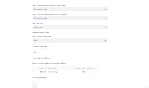## What's Next

- Adding Neural Recommneders: Unfortunately with the objective of limiting complexity of the models. Neural models based were were left out of the scope.
- Test on optimization of ads.
- Test on real ecommerces.
- Developing an Cloud SASS Recommender Engine Like Service.
- An interesting and natural progression would be to use this project and lead it into building a cloud service that simplifies and encapsulates the complexity of designing and implementation recommnedation systems
- Some competitors already in the space are:
- [SearchSpring](https://searchspring.com/?utm_medium=paid_search&utm_source=google_ads&utm_campaign=g_s_nb_namer_generic&utm_term=product%20recommendation%20software)
- [Nosto](https://www.nosto.com/commerce-experience-platform/product-recommendations/?utm_medium=paid&utm_source=google-search&utm_campaign=x_psn_ww_x_en&utm_content=cxp-product-rec_demo-request&utm_term=ecommerce%20product%20recommendation%20engine&gad_source=1&gclid=Cj0KCQjw0ruyBhDuARIsANSZ3wrYXTzbysi7EEH5mxOAmtxlN6qdv0fHZJqNX0x6XwXUxpgbajPIATcaAmjNEALw_wcB)
- [Contextly Recommends By Contextly](https://wordpress.org/plugins/contextly-related-links/)

## References

- Surprise Library Reference https://surprise.readthedocs.io/en/stable/notation_standards.html#id8

### Further Reading

- Recommender systems, a celebration of collaborative filtering and content filtering https://xuwd11.github.io/Recommender_Systems/

Multi arm badnit.
Mutoi