# Chapter 14: Mixture models
Let's take a look at marbles problem earlier:
Bag1 → `Unknown distribution` → Sample1 → Color1
Bag2 → `Unknown distribution` → Sample2 → Color2
...
BagN → `Unknown distribution` → SampleN → ColorN
Here we know deterministically that Color1 came from Bag1 and so on. What if we remove this information?
[Bag1, Bag2, ..., BagN] → `Sample bag1` → `Sample Color1`
[Bag1, Bag2, ..., BagN] → `Sample bag2` → `Sample Color2`
...
[Bag1, Bag2, ..., BagN] → `Sample bag n` → `Sample Color n`
Here we need to learn two things given some observed data:
- how are the bags distributed?
- how are colors in each bag distributed?
```javascript
var colors = ['blue', 'green', 'red']
var observedData = [{name: 'obs1', draw: 'red'},
{name: 'obs2', draw: 'red'},
{name: 'obs3', draw: 'blue'},
{name: 'obs4', draw: 'blue'},
{name: 'obs5', draw: 'red'},
{name: 'obs6', draw: 'blue'}]
var predictives = Infer({method: 'MCMC', samples: 30000}, function(){
var phi = dirichlet(ones([3, 1]))
var alpha = 1000.1
var prototype = T.mul(phi, alpha)
var makeBag = mem(function(bag){
var colorProbs = dirichlet(prototype)
return Categorical({vs: colors, ps: colorProbs})
})
// each observation (which is named for convenience) comes from one of three bags:
var obsToBag = mem(function(obsName) {return uniformDraw(['bag1', 'bag2', 'bag3'])})
var obsFn = function(datum){
observe(makeBag(obsToBag(datum.name)), datum.draw)
}
mapData({data: observedData}, obsFn)
return {sameBag1and2: obsToBag(observedData[0].name) === obsToBag(observedData[1].name),
sameBag1and3: obsToBag(observedData[0].name) === obsToBag(observedData[2].name)}
})
```
Notice how the bag is selected uniformly at random:
```javascript
var obsToBag = mem(function(obsName) {return uniformDraw(['bag1', 'bag2', 'bag3'])})
```
> Instead of assuming that a marble is equally likely to come from each bag, we could instead learn a distribution over bags where each bag has a different probability.
>
```javascript
var bagMixture = dirichlet(ones([3, 1]))
var obsToBag = mem(function(obsName) {
return categorical({vs: ['bag1', 'bag2', 'bag3'], ps: bagMixture});
})
```
---
### Example: Topic Models
Problem: Given a document (assumed to be a bag of words) and a set of topics, classify the document as one of the topics.
Approach:
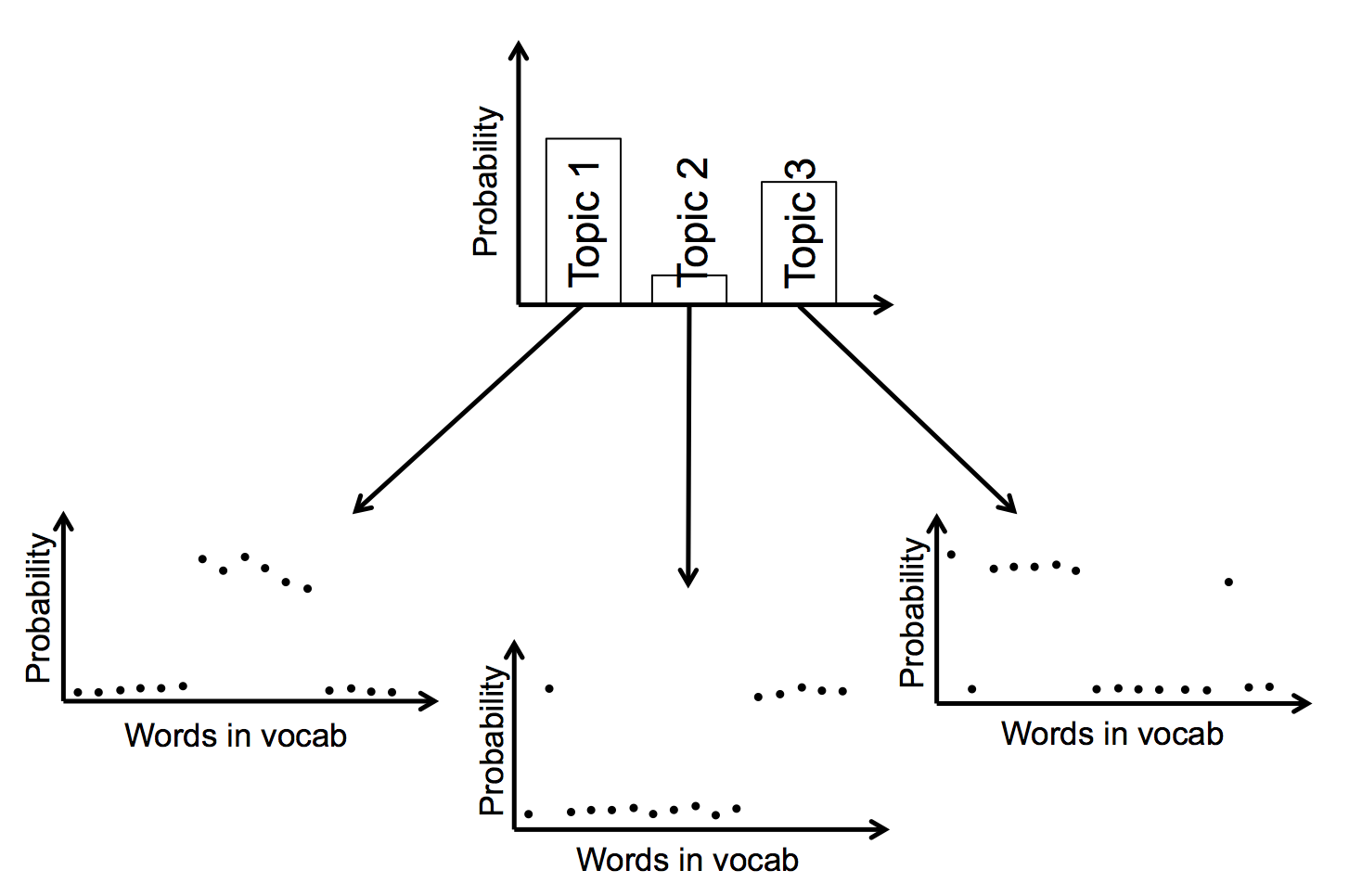
> Each topic is associated with a distribution over words, and this distribution is drawn from a Dirichlet prior.
[Vocabulary] → [Topic1]
[Vocabulary] → [Topic2]
...
[Vocabulary] → [Topic k]
> For each document, mixture weights over a set of `k` topics are drawn from a Dirichlet prior.
[Dirichlet prior] → [Topic1, Topic2, ... Topic k] for a document
> For each of the N topics (where N = length of the doc) drawn for the document, a word is sampled from the corresponding multinomial distribution.
>
For each word:<br>
[Topic1, Topic2, ... Topic k] → [Topic] → [Word] → Observe similarity with word in a document
```javascript
var expectationOver = function(topicID, results) {
return function(i) {
return expectation(results, function(v) {return T.get(v[topicID], i)})
}
}
var vocabulary = ['DNA', 'evolution', 'parsing', 'phonology'];
var eta = ones([vocabulary.length, 1])
var numTopics = 2
var alpha = ones([numTopics, 1])
var corpus = [
'DNA evolution DNA evolution DNA evolution DNA evolution DNA evolution'.split(' '),
'DNA evolution DNA evolution DNA evolution DNA evolution DNA evolution'.split(' '),
'DNA evolution DNA evolution DNA evolution DNA evolution DNA evolution'.split(' '),
'parsing phonology parsing phonology parsing phonology parsing phonology parsing phonology'.split(' '),
'parsing phonology parsing phonology parsing phonology parsing phonology parsing phonology'.split(' '),
'parsing phonology parsing phonology parsing phonology parsing phonology parsing phonology'.split(' ')
]
var model = function() {
var topics = repeat(numTopics, function() {
return dirichlet({alpha: eta})
})
mapData({data: corpus}, function(doc) {
var topicDist = dirichlet({alpha: alpha})
mapData({data: doc}, function(word) {
var z = sample(Discrete({ps: topicDist}))
var topic = topics[z]
observe(Categorical({ps: topic, vs: vocabulary}), word)
})
})
return topics
}
var results = Infer({method: 'MCMC', samples: 20000}, model)
//plot expected probability of each word, for each topic:
var vocabRange = _.range(vocabulary.length)
print('topic 0 distribution')
viz.bar(vocabulary, map(expectationOver(0, results), vocabRange))
print('topic 1 distribution')
viz.bar(vocabulary, map(expectationOver(1, results), vocabRange))
```
Intuitively what's happening here is:
- Each time we see a document, we sample a distribution over topics
- For each word, we sample a topic which should have a high probability of showing the corresponding word
Image source: [Latent Dirichlet Allocation (LDA) \| NLP-guidance](https://moj-analytical-services.github.io/NLP-guidance/LDA.html)
#### Plate notation (from wiki)
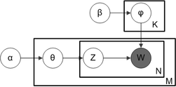
> M denotes the number of documents
> N is number of words in a given document (document i has N<sub>i</sub> words)
> α is the parameter of the Dirichlet prior on the per-document topic distributions
> β is the parameter of the Dirichlet prior on the per-topic word distribution
> θ<sub>i</sub> is the topic distribution for document i
> z<sub>ij</sub> is the topic for the j-th word in document i
---
### Example: Categorical Perception of Speech Sounds
> Human perception is often skewed by our expectations. A common example of this is called categorical perception – when we perceive objects as being more similar to the category prototype than they really are. In phonology this is been particularly important and is called the perceptual magnet effect: Hearers regularize a speech sound into the category that they think it corresponds to. Of course this category isn’t known a priori, so a hearer must be doing a simultaneous inference of what category the speech sound corresponded to, and what the sound must have been.
>
The code is simple but the implications are deep.
```javascript
var prototype1 = 0
var prototype2 = 5
var stimuli = _.range(prototype1, prototype2, 0.2)
var perceivedValue = function(stim){
return expectation(Infer({method: 'MCMC', samples: 10000}, function(){
var vowel1 = Gaussian({mu: prototype1, sigma: 1})
var vowel2 = Gaussian({mu: prototype2, sigma: 1})
var category = flip()
var value = category ? sample(vowel1) : sample(vowel2)
observe(Gaussian({mu: value, sigma: 1}),stim)
return value
}))
}
var stimulusVsPerceivedValues = map(function(s){return {x:s, y:perceivedValue(s)}}, stimuli)
viz.scatter(stimulusVsPerceivedValues)
```

Notice that the perceived value is the expectation of all values that are observed for a given `value`. This means __on average most values for a given `value` tend to be on left or right side of `value`__. This is where the skewness comes in.
---
### Unknown Numbers of Categories
In the previous examples the number of categories was fixed. But that can be problematic.
> The simplest way to address this problem, which we call unbounded models, is to simply place uncertainty on the number of categories in the form of a hierarchical prior.
> __Example__: Inferring whether one or two coins were responsible for a set of outcomes (i.e. imagine a friend is shouting each outcome from the next room–“heads, heads, tails…”–is she using a fair coin, or two biased coins?).
>
```javascript
// var observedData = [true, true, true, true, false, false, false, false]
var observedData = [true, true, true, true, true, true, true, true]
var results = Infer({method: 'rejection', samples: 100}, function(){
var coins = flip() ? ['c1'] : ['c1', 'c2'];
var coinToWeight = mem(function(c) {return uniform(0,1)})
mapData({data: observedData},
function(d){observe(Bernoulli({p: coinToWeight(uniformDraw(coins))}),d)})
return {numCoins: coins.length}
})
viz(results)
```
We can extend the idea to a higher number of bags by using a `Poisson distrbution`:
```javascript
var colors = ['blue', 'green', 'red']
var observedMarbles = ['red', 'red', 'blue', 'blue', 'red', 'blue']
var results = Infer({method: 'rejection', samples: 100}, function() {
var phi = dirichlet(ones([3,1]));
var alpha = 0.1;
var prototype = T.mul(phi, alpha);
var makeBag = mem(function(bag){
var colorProbs = dirichlet(prototype);
return Categorical({vs: colors, ps: colorProbs});
})
// unknown number of categories (created with placeholder names):
var numBags = (1 + poisson(1));
var bags = map(function(i) {return 'bag' + i;}, _.range(numBags))
mapData({data: observedMarbles},
function(d){observe(makeBag(uniformDraw(bags)), d)})
return {numBags: numBags}
})
viz(results)
```
But is the number of categories infinite here? No!
> In an unbounded model, there are a finite number of categories whose number is drawn from an unbounded prior distribution
>
An alternative is to use _infinite_ mixture models.
---
### Infinite mixture models aka Dirichlet Process
Consider the discrete probability distribution:
`[a,b,c,d]` where `a+b+c+d=1`
It can be interpreted as:
- Probability of stopping at a = `a / (a+b+c+d)`
- Probability of stopping at b = `b / (b+c+d)`
- Probability of stopping at c = `c / (c+d)`
- Probability of stopping at d = `d / (d)`
Note that the last number is always 1 and all other numbers are always between 0 and 1.
Conversely, we can convert any list with all but last entries between 0 and 1 and last entry as 1 like so:
`[p,q,r,1]` means
- Probability of stopping at first index = p
- Probability of stopping at second index = q
- Probability of stopping at second index = r
- Probability of stopping at second index = 1
Thus it could be converted into a discrete probability distribution of length 4.
But what if we never decide to stop. In other words what if all the numbers `[p,q,r,s,...]` are between 0 and 1.
Whenever we sample from this distribution, it will stop at a random index between 1 and infinity.
This can be modeled as:
```javascript
// resid = [p,q,r,s,...]
var mySampleDiscrete = function(resid,i) {
return flip(resid(i)) ? i : mySampleDiscrete(resid, i+1)
}
```
But how do we create this infinitely long array of probabilities? In other words how does one set a prior over an infinite set of bags?
```javascript
//a prior over an infinite set of bags:
var residuals = mem(function(i){uniform(0,1)}) // could also be beta(1,1) instead of uniform(0,1)
var mySampleDiscrete = function(resid,i) {
return flip(resid(i)) ? i : mySampleDiscrete(resid, i+1)
}
var getBag = mem(function(obs){
return mySampleDiscrete(residuals,0)
})
```
Thus we can construct an infinite mixture model like so:
```javascript
var colors = ['blue', 'green', 'red']
var observedMarbles = [{name:'obs1', draw: 'red'},
{name:'obs2', draw: 'blue'},
{name:'obs3', draw: 'red'},
{name:'obs4', draw: 'blue'},
{name:'obs5', draw: 'red'},
{name:'obs6', draw: 'blue'}]
var results = Infer({method: 'MCMC', samples: 200, lag: 100}, function() {
var phi = dirichlet(ones([3,1]));
var alpha = 0.1
var prototype = T.mul(phi, alpha);
var makeBag = mem(function(bag){
var colorProbs = dirichlet(prototype);
return Categorical({vs: colors, ps: colorProbs});
})
//a prior over an infinite set of bags:
var residuals = mem(function(i){uniform(0,1)})
var mySampleDiscrete = function(resid,i) {
return flip(resid(i)) ? i : mySampleDiscrete(resid, i+1)
}
var getBag = mem(function(obs){
return mySampleDiscrete(residuals,0)
})
mapData({data: observedMarbles},
function(d){observe(makeBag(getBag(d.name)), d.draw)})
return {samebag12: getBag('obs1')==getBag('obs2'),
samebag13: getBag('obs1')==getBag('obs3')}
})
```
###### tags: `probabilistic-models-of-cognition`