你所不知道的 C 語言：遞迴呼叫篇

--- tags: DYKC, CLANG, C LANGUAGE, recursion --- # [你所不知道的 C 語言](https://hackmd.io/@sysprog/c-prog/)：遞迴呼叫篇 *「[遞迴（recurse）只應天上有，凡人該當用迴圈（iterate）](http://coder.aqualuna.me/2011/07/to-iterate-is-human-to-recurse-divine.html)」* Copyright (**慣C**) 2016, 2018 [宅色夫](http://wiki.csie.ncku.edu.tw/User/jserv) ==[直播錄影](https://youtu.be/gilUlOXjLt0)== ![](https://i.imgur.com/t8YpCcs.png) A loop within a loop; A pointer to a pointer; A recursion within a recursion; ## 聖經本蘊藏的密碼 ![](https://i.imgur.com/CyRlatp.jpg) 《The C Programming Language》一書之所以被列為經典，不僅在於這是 C 語言發明者的著作，更在於不到三百頁卻涵蓋 C 語言的精髓，佐以大量範例，循序漸進。更奇妙的是，連索引頁 (index) 也能隱藏學問。上圖是《The C Programming Language》的第 269 頁，是索引頁面的一部分，注意到 recursion (遞迴)一字出現在書本的第 86, 139, 141, 182, 202, 以及 269 頁，後者恰好就是 recursion 出現的頁碼，符合遞迴的定義！ [cursive](https://www.dictionary.com/browse/cursive) vs. [recursive](https://www.dictionary.com/browse/recursive) ![](https://hackmd.io/_uploads/HJ4d6oMFs.png) > [source](https://twitter.com/memecrashes/status/1446551837495201797/photo/1) ## 遞迴讓你直覺地表示特定模式觀賞影片 [Binary, Hanoi and Sierpinski - Part I](https://www.youtube.com/watch?v=2SUvWfNJSsM) 和 [Binary, Hanoi, and Sierpinski - Part II](https://www.youtube.com/watch?v=bdMfjfT0lKk)，記得開啟 YouTube 的字幕 ![](https://i.imgur.com/4Y55fE1.png) ![](https://i.imgur.com/Gq61cAf.png) > [Tail Call Optimization: The Musical](https://youtu.be/-PX0BV9hGZY) (2019 年) 也是有趣的短片。[HackerNews 討論](https://news.ycombinator.com/item?id=26470532) 電腦程式中，副程式直接或間接呼叫自己就稱為遞迴。遞迴算不上演算法，只是程式流程控制的一種。程式的執行流程只有兩種: * 循序，分支(迴圈) * 呼叫副程式(遞迴) 迴圈是一種特別的分支，而遞迴是一種特別的副程式呼叫。不少初學者以及教初學者的人把遞迴當成是複雜的演算法，其實單純的遞迴只是另一種函數定義方式而已，在程式指令上非常簡單。初學者為什麼覺得遞迴很難呢？因為他跟人類的思考模式不同，電腦的兩種思維模式：窮舉與遞迴(enumeration and recursion)，窮舉是我們熟悉的而遞迴是陌生的，而遞迴為何重要呢？因為他是思考好的演算法的起點，例如分治與動態規劃。分治：一刀均分左右，兩邊各自遞迴，返回重逢之日，真相合併之時。分治 (Divide and Conquer) 是種運用遞迴的特性來設計演算法的策略。對於求某問題在輸入 S 的解 P(S) 時，我們先將 S 分割成兩個子集合 S~1~ 與 S~2~，分別求其解 P(S~1~) 與 P(S~2~)，然後再將其合併得到最後的解 P(S)。要如何計算 P(S~1~) 與 P(S~2~) 呢？因為是相同問題較小的輸入，所以用遞迴來做就可以了。分治不一定要分成兩個，也可以分成多個，但多數都是分成兩個。那為什麼要均分呢？從下面的舉例說明中會了解。從一個非常簡單例子來看：在一個陣列中如何找到最大值。迴圈的思考模式是：從左往右一個一個看，永遠記錄著目前看到的最大值。 ```c m = a[0]; for (i = 1 ; i < n; i++) m = max(m, a[i]); ``` 分治思考模式：如果我們把陣列在i的位置分成左右兩段 $a[0, i-1]$ 與 $a[i, n]$，分別求最大值，再返回兩者較大者。切在哪裡呢？如果切在最後一個的位置，因為右邊只剩一個無須遞迴，那麼會是 ```c int find_m1(int n) { if (n == 0) return a[0]; return max(find_m1(n - 1), a[n]); } ``` 這是個尾端遞迴 (Tail Recursion)，在有編譯最佳化的狀況下可跑很快，其實可發現程式的行為就是上面那個迴圈的版本。若我們將程式切在中點: ```c int find_m2(int left, int right) { // 範圍=[left, right) 慣用左閉右開區間 if (right - left == 1) return a[left]; int mid = (left + right) / 2 ; return max(find_m2(left, mid), find_m2(mid, right)); } ``` 效率一樣是線性時間，會不會遞迴到 stack overflow 呢？放心，如果有200 層遞迴陣列可以跑到 2^200^，地球已毀滅。再來看個有趣的問題：假設我們有一個程式比賽的排名清單，有些選手是女生有些是男生，我們想要計算有多少對女男的配對是男生排在女生前面的。若以 0 與 1 分別代表女生與男生，那麼我們有一個 0/1 序列 $a[n]$，要計算 ``` Ans = | {(a[i], a[j]) | i < j 且 a[i] > a[j]} | ``` 迴圈的思考方式：對於每一個女生，計算排在他前面的男生數，然後把它全部加起來就是答案。 ```c for (i = 0, ans = 0 ; i < n ;i++) { if (a[i]==0) { cnt = num of 1 before a[i]; ans += cnt; } } ``` 效率取決於如何計算 `cnt`。如果每次拉一個迴圈來重算，時間會跑到 $O(n^2)$，如果利用類似前綴和 (prefix-sum) 的概念，只需要線性時間。 ```c for (i = 0, cnt = 0, ans = 0 ; i <n ;i++) { if (a[i] == 0) ans += cnt; else cnt++; } ``` 接下來看分治思考模式。如果我們把序列在 i 處分成前後兩段 $a[0, i-1]$ 與 $a[i, n]$，任何一個要找的 (1, 0) 數對只可能有三個可能：都在左邊、都在右邊、或是一左一右。所以我們可左右分別遞迴求，對於一左一右的情形，我們若知道左邊有 x 個 1 以及右邊有 y 個 0，那答案就有 xy 個。遞迴終止條件是什麼呢？剩一個就不必找下去。 ```c int dc(int left, int right) { // 範圍=[left,right) 慣用左閉右開區間 if (right - left < 2) return 0; int mid = (left + right) / 2; // 均勻分割 int w = dc(left, mid) + dc(mid, right); 計算x = 左邊幾個 1, y = 右邊幾個 0 return w + x * y; } ``` 時間複雜度呢？假設把範圍內的資料重新看一遍去計算 0 與 1 的數量，那需要線性時間，整個程序的時間變成 $T(n) = 2T(n/2) + O(n)$，結果是 $O(n\log{}n)$，不好。比迴圈的方法差，原因是因為我們計算 0/1 的數量時重複計算。我們讓遞迴也回傳 0 與 1 的個數，效率就會改善了，用 Python 改寫： ```python def dc(left, right): if right - left == 1: if ar[left]==0: return 0, 1, 0 # 逆序數，0的數量，1的數量 return 0, 0, 1 mid = (left + right) // 2 #整數除法 w1, y1, x1 = dc(left,mid) w2, y2, x2 = dc(mid,right) return w1 + w2 + x1 * y2, y1 + y2, x1 + x2 ``` 時間效率是 $T(n) = 2T(n/2) + O(1)$，所以結果是 $O(n)$。如果分治可以做的迴圈也可以，那又何必學分治？第一，複雜的問題不容易用迴圈的思考找到答案；第二，有些問題迴圈很難做到跟分治一樣的效率。上述男女對的問題其實是逆序數對問題的弱化版本：給一個數字序列，計算有多少逆序對，也就是 ``` | {(a[i], a[j]) | i < j 且 a[i] > a[j]} |。 ``` 迴圈的思考模式一樣去算每一個數字前方有多少大於它的數，直接做又搞到O(n^2)，有沒有辦法像上面男女對問題一樣，紀錄一些簡單的資料來減少計算量呢？你或許想用二分搜，但問題是需要重排序，就我所知，除非搞個複雜的資料結構，否則沒有簡單的辦法可以來加速。那麼來看看分治。基本上的想法是從中間切割成兩段，各自遞迴計算逆序數並且各自排序好，排序的目的是讓合併時，對於每個左邊的元素可以笨笨地運用二分搜去算右邊有幾個小於它。 ```c LL sol(int le, int ri) { // 區間 = [le,ri) if (ri-le == 1) return 0; int mid = (ri + le) / 2; LL w = sol(le, mid) + sol(mid, ri); LL t = 0; for (int i = le; i < mid; i++) t += lower_bound(ar + mid, ar + ri, ar[i]) - (ar + mid); sort(ar + le, ar + ri); return w + t; } ``` 時間複雜度呢？即使我們笨笨地把兩個排好序的序列再整個重排，$T(n) = 2T(n/2) + O(n\log{}n)，$結果是 O(nlog~2~(n))，十萬筆資料不需要一秒，比迴圈的方法好多了。為什麼說笨笨地二分搜尋與笨笨地重新排序呢？對於兩個排好序的東西要合併其實可以用線性時間。那二分搜呢？沿路那麼多個二分搜其實可以維護兩個註標一路向右就好了。所以事實上不需要複雜的資料結構可以做到 $O(n\log{}n)$，熟悉演算法的人其實看得出來，這個方法基本上就是很有名的 merge sort，跟 quick sort 一樣常拿來當作分治的範例。另外，如果merge sort的分割方式如果是 $[left, right-1]$ $[right-1, right]$，右邊只留一個，那就退化成 insertion sort 的尾端遞迴。註：計算遞迴的時間需要解遞迴函數，這是有點複雜的事情。好在大多數常見的有公式解。 Tail recursion 是遞迴的一種特殊形式，副程式只有在最後一個動作才呼叫自己。以演算法的角度來說，recursion tree 全部是一脈單傳，所以時間複雜度是線性個該副程式的時間。不過遞迴是需要系統使用 stack 來儲存某些資料，於是還是會有 stack overflow 的問題。但是從編譯器的角度來說，因為最後一個動作才呼叫遞迴，所以很多 stack 資料是沒用的，所以他是可以被優化的。基本上，優化以後就不會有時間與空間效率的問題。注意: Python 沒有 tail recursion 優化，而且 stack 深度不到 1000。C 要開編譯器開啟最佳化才會做 tail recursion 優化。延伸閱讀: * [On Recursion, Continuations and Trampolines](https://eli.thegreenplace.net/2017/on-recursion-continuations-and-trampolines/) ## 遞迴程式沒有你想像中的慢得益於現代的編譯器最佳化技術，遞迴的程式不見得會比迭代 (iterative) 的版本來得慢。以找最大公因數 (Greatest Common Divisor，縮寫 GCD) 來說，典型的演算法為輾轉相除法，又稱歐幾里得算法 (Euclidean algorithm)，考慮以下兩種實作 - [ ] 遞迴的實作 ```c unsigned gcd_rec(unsigned a, unsigned b) { if (!b) return a; return gcd_rec(b, a % b); } ``` - [ ] 迭代的實作 ```c unsigned gcd_itr(unsigned a, unsigned b) { while (b) { unsigned tmp = b; b = a % b; a = tmp; } return a; } ``` 分析 clang/llvm 編譯的輸出 (參數 `-S -O2`)，不難發現兩者轉譯出的 inner loop 的組合語言完全一樣: ``` LBB0_2: movl %edx, %ecx xorl %edx, %edx divl %ecx testl %edx, %edx movl %ecx, %eax jne LBB0_2 ``` 顯然遞迴版本的原始程式碼簡潔，而且對應於輾轉相除法的數學定義。延伸閱讀: [遞迴 (Recursion)](https://notfalse.net/9/recursion) ## 案例分析: 等效電阻幾個連接起來的電阻所起的作用，可以用一個電阻來代替，這個電阻就是那些電阻的等效電阻。也就是說任何電迴路中的電阻，不論有多少只，都可等效為一個電阻來代替。而不影響原迴路兩端的電壓和迴路中電流強度的變化。這個等效電阻，是由多個電阻經過等效串並聯公式，計算出等效電阻的大小值。也可以說，將這一等效電阻代替原有的幾個電阻後，對於整個電路的電壓和電流量不會產生任何的影響，所以這個電阻就叫做迴路中的等效電阻。 ``` r r r -----###-----------###----------- . . . --------###------------- A | | | | | # # # # # r # r # r # # r # # # # # # | | | | | ---------------------------------- . . . ------------------------ B 1 2 3 n - 1 ``` (a) ``` r ----------###------------- A -------- A | | | # # # R(r, n - 1) # r # ==> # R(r, n) # # # | | | --------------------------- B -------- B ``` (b) Fig: Decomposition of the ladder of resistors problem, and deivation of the recursive case through induction When they are connected in parallel the new resistance is $r = ({r1}\times{r2})/({r1}+{r2})$. Alternatively, it can be expressed as: $$\frac1r = \frac1{r1} + \frac1{r2}$$ These rules can be applied successively to pairs of resistors until we obtain a circuit that contains a single resistor. However, this process is tedious. Instead, recursion provides a succinct and elegant solution. The problem has two input parameters: the resistance $( r )$ and the number of rungs $( n )$ of the ladder. The size of the problem is clearly $n$ ($r$ plays a role in the final value, but is not responsible for the runtime of the algorithm). Let $R(r,n)$ denote the recursive function. The base case occurs when $n = 1$, where the initial ladder would only contain a single resistor. Therefore in that case $R(r, 1) = r$. For the recursive case we need to find a subproblem within the original with exactly the same structure. Figure 4.6(a) shows the decomposition of the problem by decrementing its size by a unit. The circuit associated with the subproblem can be replaced by a single resistor of resistence $R(r, n - 1)$, as shown in (b), where we can assume that we know its value by using induction. Finally, it is fairly straightforward to simplify the resulting circuit that contains only three resistors. Firstly, the left and top resistors are connected in series. Thus, they can be merged to form a resistor with resistance $R(r, n - 1) + r$. Finally, this new resistor is connected in parallel to the right resistor. $R(r, n)$ can be defined through: $$\frac{1}{R(r,n)} = \frac1r + \frac1{R(r, n - 1) + r}$$ The recursive function is therefore: $$ R(r,n)= \begin{cases} r & \text{if n = 1}\\ 1 / (\frac1r + \frac1{R(r, n - 1) + r}) & \text{if n > 1} \end{cases} $$ Finally, as a curious note, it is possible to show that $R(r,n) = rF(2n - 1)/F(2n)$, where $F$ is the Fibonacci function. - Function that solves the ladder of resistors problem: ```python def circuit(n, r): if n == 1: return r else: return 1 / (1 / r + 1 / (circuit(n - 1, r) + r)) ``` ## 案例分析：數列輸出以下 C 程式的作用為何？ ```c= int p(int i, int N) { return (i < N && printf("%d\n", i) && !p(i + 1, N)) || printf("%d\n", i); } ``` 拆解為以下兩部份: - [ ] Line `#2` ```clike=2 (i < N && printf("%d\n", i) && !p(i + 1, N)) ``` * 依據 [C Operator Precedence](http://en.cppreference.com/w/c/language/operator_precedence)，`&&` (Logical AND) operator 的運算規則為左值優先，只要左值不成立，右值都不會執行 * 因此我們可確定，當 `i` 不小於 `N` 時，不會印出 `i`，也不會呼叫 `p` * [printf(3)](https://linux.die.net/man/3/printf) 會回傳印出的字元數目，這裡一定回傳非零值 * 接著我們可推斷，當 `i < N` 成立，`i` 會被輸出，接著會呼叫 `p` * 換言之，中止條件是 `i >= N` :::info 查詢 man page，對應到 GNU/Linux 的命令為 `man 3 printf` ::: - [ ] Line `#3` ```clike=3 || printf("%d\n", i) ``` * `||` (Logical OR) operator 的運算規則為當左值成立時，右值就不會執行 * 因此 `p` 前面的 `!` 很重要。因為 p 的回傳值一定是 true (由於 `printf` 一定回傳非零值)，而為確保會執行到這第二個 `printf`，要將回傳值作 NOT，讓第一部份的結果為 false * 如果去掉 NOT，則只會輸出 `i -> N` :::info 把 `!p(i+1, N)` 的反相`!` 拿掉後，得到以下結果: ``` /* i = 1 , n = 5 */ 1 2 3 4 5 ``` ::: * 第二個 `printf` 要等 `p` 執行完畢才會被執行。遞迴呼叫在實作層面來說，就是藉由 stack 操作，這裡一旦被 push 到 stack 印一次，被 pop 出來再印一次綜合以上分析，我們可得知上述程式碼的作用為「印出 i -> N -> i 的整數序列，N 只會出現一次」。延伸問題: 把 `&&` 前後的敘述對調，是否影響輸出？ * 也就是說，變更原始程式碼，從 `i < N && printf("%d\n", i)` 改為 `printf("%d\n", i) && (i < N)` 的話 * 如果對調 `printf` 跟 `i < N` 則會輸出 `i -> N N -> i` (N 出現兩次) * 因為 `printf` 會先被執行，不會受到 `i < N` 成立與否影響。 * 延伸問題：`i` 和 `N` 組合的有效上下界為何？ * 科技公司的面試過程中，這類題目有助於測驗應試者的系統概念 * 不妨將原本程式碼改寫為以下： ```c #include <limits.h> #include <stdio.h> int p(int i, int N) { return (i < N && printf("%d\n", i) && !p(i + 1, N)) \ || printf("%d\n", i); } int main() { return p(0, INT_MAX); } ``` * 在 Linux x86_64 環境編譯並執行後，會得到類似以下輸出: (數字可能會有出入) ``` 261918 261919 261920 程式記憶體區段錯誤 ``` * 這裡的 segmentation fault 意味著 stack overflow，遞迴呼叫時，每一層都有變數存放於 stack 中，每次呼叫也要保存回傳位址 (return address) :::info 可用 `ulimit -s` 來改 stack size，預設是 8 MB，計算後可推得，每個 stack 大約佔用 32 bytes，N 的限制取決於 stack size 的數值。延伸閱讀: [通過 ulimit 改善系統效能](https://www.ibm.com/developerworks/cn/linux/l-cn-ulimit/) ::: * 複習 [你所不知道的C語言：函式呼叫篇](https://hackmd.io/s/SJ6hRj-zg)，我們知道為了滿足 [x86_64 ABI / calling convention](https://en.wikipedia.org/wiki/X86_calling_conventions)，回傳位址佔 8 bytes, (int) `i` 和 (int) `N` 這兩個變數合計 8 bytes, 函式的區域變數 (給 `printf()` 用的 format string 的位置) 8 bytes, p 回傳值 int 佔 4bytes ，總共 32 bytes。計算過程: ``` 8MB = 8,388,608 bytes 8,388,608 / 32 = 262,144 次 ``` * 綜合上述，推算出 `0 < N - i < 262144` * 實驗 (檔名為 `p.c`) ```shell $ gcc -o p p.c -g $ gdb -q p Reading symbols from p...done. (gdb) break p Breakpoint 1 at 0x6ae: file p.c, line 7. (gdb) run Starting program: /tmp/p Breakpoint 1, p (i=0, N=2147483647) at p.c:7 7 || printf("%d\n", i); (gdb) info frame Stack level 0, frame at 0x7fffffffdf60: rip = 0x5555555546ae in p (p.c:7); saved rip = 0x555555554721 called by frame at 0x7fffffffdf70 source language c. Arglist at 0x7fffffffdf50, args: i=0, N=2147483647 Locals at 0x7fffffffdf50, Previous frame's sp is 0x7fffffffdf60 Saved registers: rbp at 0x7fffffffdf50, rip at 0x7fffffffdf58 ``` :::warning 現代編譯器的最佳化可能會造成非預期的改變，比方說在前述編譯參數追加 `-O3`，在 gcc-6.2 輸出的執行檔會得到以下輸出: 523637 523638 523639 程式記憶體區段錯誤 ::: ![](https://i.imgur.com/Zzl8fYg.png) [ [source](https://twitter.com/ProductHunt/status/1013695862508097536) ] ## 遞迴程式設計 * [Recursive Programming](https://web.archive.org/web/20191228141133/http://www.cs.cmu.edu:80/~adamchik/15-121/lectures/Recursions/recursions.html) * [Recursive Functions](https://web.archive.org/web/20171116063115/http://www.cs.umd.edu:80/class/fall2002/cmsc214/Tutorial/recursion2.html) ## Fibonacci sequence 數學定義如下: $F_n = F_{n-1}+F_{n-2},$ $F_0 = 0, F_1 = 1$ 數列值： | $F_0$ | $F_1$ | $F_2$ | $F_3$ |$F_4$|$F_5$|$F_6$|$F_7$|$F_8$|$F_9$|$F_{10}$|$F_{11}$|$F_{12}$|$F_{13}$|$F_{14}$|$F_{15}$|$F_{16}$|$F_{17}$| $F_{18}$|$F_{19}$|$F_{20}$| | ----| ---- | ---- |---- |---- |---- |---- |---- |---- |---- |---- |---- |---- |---- |---- |---- |---- |---- |---- |---- |---- | | 0| 1 |1|2|3|5|8|13|21|34|55|89|144|233|377|610|987|1597|2584|4181|6765| 在 Fibonacci 數列上其解法可分為下列 * 遞迴法 * 非遞迴法 * [近似解](https://www.mathsisfun.com/numbers/fibonacci-sequence.html) * [線性代數解](https://en.wikibooks.org/wiki/Linear_Algebra/Topic:_Linear_Recurrences) * [排列組合解](http://yqcmmd.com/2015/06/23/fibonacci/) 此數列的解法非常多元。下段我們選出幾種經典實作。 ### 遞迴法 (Recursive) 即是 Fibonacci 數列定義，將此轉為程式碼 ```c int fib(int n) { if (n == 0) return 0; if (n == 1) return 1; return fib(n - 1) + fib (n - 2); } ``` ### 非遞迴法 (Iterative) 可縮減原先使用遞迴法的函式呼叫造成之執行時期開銷。以下先討論基本方法。 ```c int fib(int n) { int pre = -1; int result = 1; int sum = 0; for (int i = 0; i <= n; i++) { sum = result + pre; pre = result; result = sum; } return result; } ``` 我們可減少變數的使用： ```c int fib(int n) { int pre = -1; int i = n; n = 1; int sum = 0; while (i > 0) { i--; sum = n + pre; pre = n; n = sum; } return n; } ``` ### Tail recursion 此法可加速原先之遞迴，可減少一半的資料回傳，而概念上是運用從第一次 call function 後即開始計算值，不像之前的遞迴需 call function 至中止條件後才開始計算值，再依序傳回到最上層，因此可大幅降低時間，減少 stack 使用量。參考實作如下： ```c int fib(int n, int a, int b) { if (n == 0) return a; return fib(n - 1 , b, a + b); } ``` 此外，我們用樹狀圖來解釋 Recursive Method 以及 Tail Recursion 之差別，以下以 Fib(5) 為例。 - [ ] Recursive Method ```graphviz digraph hierarchy { graph [nodesep="1"]; 11 [label="Fib(5)" shape=box]; 21 [label="Fib(4)" shape=box]; 22 [label="Fib(3)" shape=box]; 31 [label="Fib(3)" shape=box]; 32 [label="Fib(2)" shape=box]; 33 [label="Fib(2)" shape=box]; 34 [label="Fib(1)=1" shape=box]; 41 [label="Fib(2)" shape=box]; 42 [label="Fib(1)=1" shape=box]; 43 [label="Fib(1)=1" shape=box]; 44 [label="Fib(0)=0" shape=box]; 45 [label="Fib(1)=1" shape=box]; 46 [label="Fib(0)=0" shape=box]; 51 [label="Fib(1)=1" shape=box]; 52 [label="Fib(0)=0" shape=box]; 11 ->{21 22} 21 ->{31 32} 22 ->{33 34} 31 -> {41 42} 32 -> {43 44} 33 -> {45 46} 41 -> {51 52} } ``` - [ ] Tail Recursion ```graphviz digraph hierarchy { nodesep=1.0 // increases the separation between nodes node [fontname=Courier,shape=box] //All nodes will this shape and colour "Fib(5,0,1)"->"Fib(4,1,1)" "Fib(4,1,1)"->"Fib(3,1,2)" "Fib(3,1,2)"->"Fib(2,2,3)" "Fib(2,2,3)"->"Fib(1,3,5)" "Fib(1,3,5)"->"return 5" } ``` 在兩張樹狀圖之顯示下，可明顯看出複雜度之不同，一則會發展出樹狀結構，而另一則是有如迴圈。 ### Q-Matrix $A^1 = \left( \begin{array}{ccc} 1 & 1 \\ 1 & 0 \\ \end{array} \right) = \left( \begin{array}{ccc} F_2 & F_1 \\ F_1 & F_0 \\ \end{array} \right)$ $\begin{split} A^{n+1} &= AA^n \\ &= \left( \begin{array}{ccc} 1 & 1 \\ 1 & 0 \\ \end{array} \right) \left( \begin{array}{ccc} F_{n+1} & F_{n} \\ F_{n} & F_{n-1} \\ \end{array} \right) \\ \\ &= \left( \begin{array}{ccc} F_{n+1}+F_{n} & F_{n}+F_{n-1} \\ F_{n+1} & F_{n} \\ \end{array} \right) \\ \\ &= \left( \begin{array}{ccc} F_{n+2} & F_{n+1} \\ F_{n+1} & F_{n} \\ \end{array} \right) \end{split}$ 透過矩陣轉換之方法，我們把原本之遞迴式轉換到矩陣表示，並透過矩陣次方之Divide and Conquer Method 來做加速。 $A^{2n+1} =A^{n+1}A^n$ 因此能大幅減少運算量，但此方法牽涉除法以及矩陣，其中除法可使用右移以及可利用最後一個 bit 來判斷奇偶數。實作 Fibonacci 數列如下。 ```c int **matrix_multiply(int a[2][2],int b[2][2]) { int *t = malloc(sizeof(int) * 2 * 2); memset(t, 0, sizeof(int) * 2 * 2); for (int i = 0 ; i < 2 ; i ++ ) for (int j = 0 ; j < 2 ; j ++ ) for (int k = 0 ; k < 2 ; k ++) t[i][j] += a[i][k] * b[k][j]; return t; } // 使用 Divide-and-Conquer 方法加速矩陣次方 int **matrix_pow(int a[2][2] , int n) { if (n == 1) return a; if (n % 2 == 0) { int t[2][2]; t = matrix_pow(a , n >> 1); return matrix_multiply(t , t); } int t1[2][2], t2[2][2]; t1 = matrix_pow(a, n >> 1); t2 = matrix_pow(a, (n >> 1) + 1); return matrix_multiply(t1, t2); } ``` 我們可在 Q-Matrix 的基礎上，計算 Fibonacci 數列: ```c int fib(int n) { if (n < = 0) return 0; int A1[2][2] = { { 1 , 1 } , { 1 , 0 } }; int result[2][2]; result = matrix_pow(A1, n); return result[0][1]; } ``` ### Fast doubling 此方法類似上述提及之 Q-Matrix 做法，基於矩陣之方法繼續推演而得，在效能上更勝 Q-Matrix 一籌，此概念是使用矩陣乘法相將兩個 n 次方矩陣相乘而得。 $\begin{bmatrix} 1 & 1 \\ 1 & 0 \end{bmatrix}^n = \begin{bmatrix} F(n+1) & F(n) \\ F(n) & F(n-1) \end{bmatrix}$ $\begin{split} \begin{bmatrix} F(2n+1) \\ F(2n) \end{bmatrix} &= \begin{bmatrix} 1 & 1 \\ 1 & 0 \end{bmatrix}^{2n} \begin{bmatrix} F(1) \\ F(0) \end{bmatrix}\\ \\ &= \begin{bmatrix} 1 & 1 \\ 1 & 0 \end{bmatrix}^n \begin{bmatrix} 1 & 1 \\ 1 & 0 \end{bmatrix}^n \begin{bmatrix} F(1) \\ F(0) \end{bmatrix}\\ \\ &= \begin{bmatrix} F(n+1) & F(n) \\ F(n) & F(n-1) \end{bmatrix} \begin{bmatrix} F(n+1) & F(n) \\ F(n) & F(n-1) \end{bmatrix} \begin{bmatrix} 1 \\ 0 \end{bmatrix}\\ \\ &= \begin{bmatrix} F(n+1)^2 + F(n)^2\\ F(n)F(n+1) + F(n-1)F(n) \end{bmatrix} \end{split}$ 透過上述之數學推論，我們最後可得兩公式可供使用。 $\begin{split} F(2k) &= F(k)[2F(k+1) - F(k)] \\ F(2k+1) &= F(k+1)^2+F(k)^2 \end{split}$ 接著我們即可使用此公式來撰寫 Fibonacci 數列: ```c int fib(int n) { if (n == 0) return 0; int t0 = 1; // F(n) int t1 = 1; // F(n + 1) int t3 = 1; // F(2n) int t4; // F(2n+1) int i = 1; while (i < n) { if ((i << 1) <= n) { t4 = t1 * t1 + t0 * t0; t3 = t0 * (2 * t1 - t0); t0 = t3; t1 = t4; i = i << 1; } else { t0 = t3; t3 = t4; t4 = t0 + t4; i++; } } return t3; } ``` **演算法比較** 在以上之方法中，我們比較這些方法所花費之複雜度如下，可發現最基礎之Recursive 方法是極沒效率之方法，而其後之 Q-Matrix 及 Fast Doubling 效能則有顯著差異。 | 方法 | 複雜度 | | -------- | -------- | | Recursive | $O(2^n)$ | | Iterative | $O(n)$ | | Tail Recursion | $O(n)$ | | Q-Matrix | $O(log\ n)$ | | Fast Doubling | $O(log\ n)$ | 因改良後的時間複雜度皆為同等級，我們接著實際比較執行時間。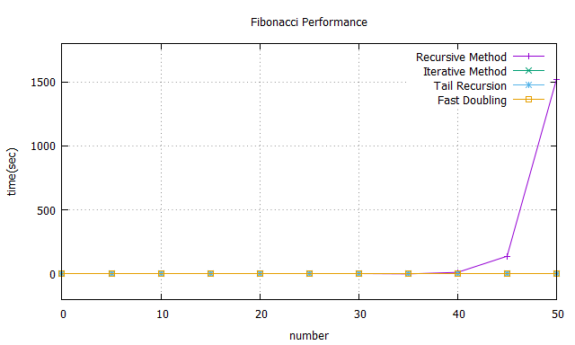 ![](https://hackpad-attachments.s3.amazonaws.com/mimihalo.hackpad.com_aqgx9ysllS2_p.478178_1443713231183_undefined) 比較 Recursive Method 和 Iterative Method 的效能差異。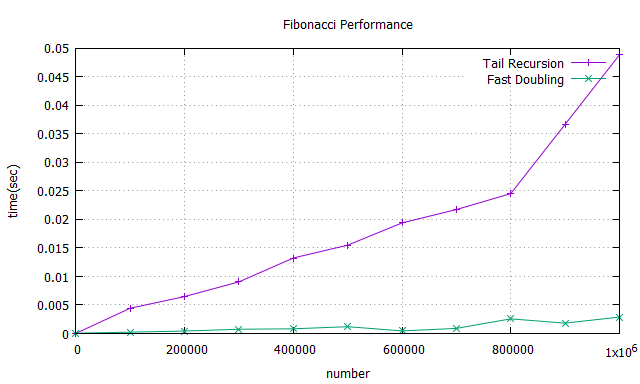 ![](https://hackpad-attachments.s3.amazonaws.com/mimihalo.hackpad.com_aqgx9ysllS2_p.478178_1443715574108_undefined) 此兩種方法在 n = 1M 時還是都有不錯的表現，與原先之 Recusive method 相比實為甚廣，而透過此兩者之比較，最後還是可得出透過Fast Doubling 的方法能得到更好之效能，對上面之複雜度圖表也能互相呼應。 Fibonacci 參考資料 * [Fibonacci number](https://en.wikipedia.org/wiki/Fibonacci_number) * [Tail call](https://en.wikipedia.org/wiki/Tail_call) * [Fibonacci Q-Matrix](http://mathworld.wolfram.com/FibonacciQ-Matrix.html) * [How to prove Fibonacci sequence with matrices?](http://math.stackexchange.com/questions/784710/how-to-prove-fibonacci-sequence-with-matrices) * [The Fibonacci Q-matrix](https://youtu.be/lTHVwsHJrG0) * [Fast Fibonacci algorithms](http://www.nayuki.io/page/fast-fibonacci-algorithms) * [Need help understanding Fibonacci Fast Doubling Proof](http://math.stackexchange.com/questions/1124590/need-help-understanding-fibonacci-fast-doubling-proof) * [An integer formula for Fibonacci numbers](https://blog.paulhankin.net/fibonacci/) ## 案例分析：字串反轉 :::success :warning: 據說某些 M 開頭的科技公司面試很喜歡出這題 ::: * 要求：用 C 語言實作 `char *reverse(char *s)`，反轉 NULL 結尾的字串，限定 in-place 與遞迴 * 先思考實作 swap 的技巧，考慮以下程式碼： ```clike void swap(int *a, int *b) { int t = *a; *a = *b; *b = t; } ``` 能否避免使用區域變數 t？又，可否改用 bit-wise operator 來改寫？ * 數值運算：利用兩個相差距離做運算，但若遇到一個很大的整數與一個負數(足夠讓他超過最大整數)兩個相減時，會產生溢位 ```clike *a = *a - *b; /* 兩數相差 */ *b = *a + *b; /* 相加得出 *b */ *a = *b - *a; /* 相減得出 *a */ ``` * 邏輯運算：運用邏輯運算查看出兩個不同相差的位元，依據以下真值表： | A | B | $\oplus$ | | -------- | -------- | -------- | | F | F | F | | F | T | T | | T | F | T | | T | T | F | ```c *a = *a ^ *b; // 求得相差位元 *b = *a ^ *b; // 與相差位元做 XOR 得出 *a *a = *a ^ *b; // 與相差位元做 XOR 得出 *b ``` 邏輯運算的好處是，可避免前述算術會遇到的 integer overflow，而且不限定位元數參考的 in-place string reverse 想法：一直 swap '\0'之前的character，演算法描述: 1. 先把首尾互換 ![](https://i.imgur.com/X0d2SxY.png) 2. 把尾端和'\0'互換 ![](https://i.imgur.com/bEB8Bt5.png) 3. 重複遞迴，直到'\0'在中間 ![](https://i.imgur.com/BpX1VrP.png) 4. 層層把'\0'換回最尾即可 ![](https://i.imgur.com/A94cmup.png) 過程示意: :::info a b c ==d== ==e== -> a b c ==e== ==d== a b ==c== ==e== d -> a b ==e== ==c== d a b e ==c== ==d== -> a b e ==d== ==c== a ==b== ==e== d c -> a ==e== ==b== d c a e b ==d== ==c== -> a e b ==c== ==d== a e ==b== ==c== d -> a e ==c== ==b== d a e c ==b== ==d== -> a e c ==d== ==b== ==a== ==e== c d b -> ==e== ==a== c d b e a ==c== ==d== b -> e a ==d== ==c== b e a d ==c== ==b== -> e a d ==b== ==c== e ==a== ==d== b c -> e ==d== ==a== b c e d a ==b== ==c== -> e d a ==c== ==b== e d ==a== ==c== b -> e d ==c== ==a== b e d c ==a== ==b== -> e d c ==b== ==a== ::: 關於這個遞迴，有更直覺的思考模式。根據題目給定， $reverse(s)$ 的作用為將 s 反轉。假設我們要反轉： $5\space 4\space 3\space 2\space 1\space$ 步驟可以分成三步，第一步是利用 $reverse(s + 1)$ 先反轉後4個： $5\space 1\space 2\space 3\space 4\space$ 然後再把1跟5對調： $1\space 5\space 2\space 3\space 4\space$ 為了讓後 4 個能再利用 $reserve(s + 1)$ 反轉，我們必須先將後三個調轉，也就是呼叫 $reverse(s+2)$： $1\space 5\space 4\space 3\space 2\space$ 這樣一來我們就能呼叫 $reverse(s+1)$ 來反轉後 4 個： $1\space 2\space 3\space 4\space 5\space$ 因此 $reverse(s)$ 可拆成以下步驟： $reverse(s+1) \to swap(s, s+1) \to reverse(s+2) \to reverse(s+1)$ 剩下就是終止條件判斷。 ```c static inline void swap(char *a, char *b) { *a = *a ^ *b; *b = *a ^ *b; *a = *a ^ *b; } char *reverse(char *s) { if ((*s == '\0') || (*(s + 1) == '\0')) return NULL; reverse(s + 1); swap(s, (s + 1)); if (*(s + 2) != '\0') reverse(s + 2); reverse(s + 1); } ``` 缺點：時間複雜度為 $T(n) = O(n^2)$ 改進思路：計算字串長度時，即可交換字元。 ```c int rev_core(char *head, int idx) { if (head[idx] != '\0') { int end = rev_core(head, idx + 1); if (idx > end / 2) swap(head + idx, head + end - idx); return end; } return idx - 1; } char *reverse(char *s) { rev_core(s, 0); return s; } ``` 時間複雜度降為 $T(n) = O(n)$ ## 案例分析: 建立目錄 [mkdir](https://man7.org/linux/man-pages/man1/mkdir.1.html) 是符合 POSIX 規範的作業系統 (如 GNU/Linux) 都有提供的工具程式，其中有項參數 `-p`: > no error if existing, make parent directories as needed 於是我們可執行命令 `mkdir -p /tmp/aaa/bbb/ccc` 來建立 `/tmp` 目錄下的 `aaa` 目錄，後者裡頭又包含 `bbb` 目錄，而 `bbb` 目錄則包含 `ccc` 目錄。 [mkdir](https://man7.org/linux/man-pages/man2/mkdir.2.html) 系統呼叫可建立新的目錄，但卻不像上述 `-p` 參數這麼方便，這時我們就可搭配遞迴呼叫的技巧來實作。程式碼如下: ```c #include <dirent.h> #include <errno.h> #include <fcntl.h> #include <stdio.h> #include <stdlib.h> #include <string.h> #include <sys/stat.h> int mkdir_r(const char *path, int level) { int ret = -1; if (!strlen(path)) goto leave; const char *c = path; int cur_level = 0; while (cur_level <= level) { for (; *c && *c != '\\' && *c != '/'; c++) /* seek for separator */ ; if (*c) c++; cur_level++; } const size_t sz = c - path + 1; char *dir = malloc(sz); if (!dir) goto leave; memcpy(dir, path, sz - 1); dir[sz - 1] = '\0'; DIR *d = opendir(dir); if (!d && mkdir(dir, S_IRWXU | S_IRWXG | S_IROTH | S_IXOTH)) { perror("mkdir"); goto leave; } if (*c) mkdir_r(path, cur_level); /* No more levels left */ ret = 0; leave: free(dir); if (d) closedir(d); return ret; } int main() { mkdir_r("aaa/bbb/ccc", 0); return 0; } ``` ## 案例分析: 類似 find 的程式 * 給定 [opendir(3)](http://man7.org/linux/man-pages/man3/opendir.3.html) 與 [readdir(3)](http://man7.org/linux/man-pages/man3/readdir.3.html) 函式，用遞迴寫出類似 [find](https://man7.org/linux/man-pages/man1/find.1.html) 的程式 * find 的功能：列出包含目前目錄和其所有子目錄之下的檔案名稱 ```c #include <sys/types.h> #include <dirent.h> void list_dir(const char *dir_name) { DIR *d = opendir(dir_name); if (!d) return; /* fail to open directory */ while (1) { struct dirent *entry = readdir(d); if (!entry) break; const char *d_name = entry->d_name; printf ("%s/%s\n", dir_name, d_name); if ((entry->d_type & DT_DIR) && strcmp(d_name, "..") && strcmp(d_name, ".")) { char path[PATH_MAX]; int path_length = snprintf(path, PATH_MAX, "%s/%s", dir_name, d_name); printf ("%s\n", path); if (path_length >= PATH_MAX) return; /* Recursively call "list_dir" with new path. */ list_dir (path); } } if (closedir (d)) return; } ``` * 練習: 如何連同檔案一併列印？ * 練習：上述程式碼實作有誤，額外的 `.` 和 `..` 也輸出了，請修正 source: [rd.c](https://www.lemoda.net/c/recursive-directory/rd.c) ## 案例分析: Merge Sort * [Program for Merge Sort in C](http://www.thecrazyprogrammer.com/2014/03/c-program-for-implementation-of-merge-sort.html): 內含動畫 * [非遞迴的版本](http://stackoverflow.com/questions/1557894/non-recursive-merge-sort) ![](https://i.imgur.com/XqHJUHw.gif) * [Merge Sort](http://www.personal.kent.edu/~rmuhamma/Algorithms/MyAlgorithms/Sorting/mergeSort.htm): 複雜度分析 * 進行中: [MapReduce with POSIX Thread](https://hackmd.io/s/Hkb-lXkyg) ## 案例分析: Bubble Sort * [Bubble Sort](http://faculty.salina.k-state.edu/tim/CMST302/study_guide/topic7/bubble.html): non-recursive vs. recursive ## 函數式程式開發 * Functional programming 在 [concurrency 環境](https://hackmd.io/s/H10MXXoT) 變得日益重要 * [Functional C](https://pdfs.semanticscholar.org/31ac/b7abaf3a1962b27be9faa2322038d1ac9ed7.pdf) * [Functional programming in C](https://lucabolognese.wordpress.com/2013/01/04/functional-programming-in-c/) * [Functional Programming 風格的 C 語言實作](https://hackmd.io/@sysprog/HyS-9S6OE) ## 遞迴背後的理論 [Lambda-calculus models of programming languages](https://dspace.mit.edu/handle/1721.1/64850) (1969 年) 指出: * 遞迴和資料型態 > "We view the work presented in this dissertation as a semantic analysis of the two subjects, recursion and data types. We tend to understand these subjects pragmatically. When a programner thinks of recursion, he thinks of push-down stacks and other aspects of how recursion "works". Similarly, types and type declarations are often described as communications to a compiler to aid it in allocating storage, etc.” * 由遞迴關係定義的函式，可視作函數式程式設計 > "Specifically, in Chapter 3 we show how a function defined by recursion can be viewed as the result of a particular operation on an object called a functional. In Chapter 4 we outline a type declaration system in which a type can be construed as a set of objects and a type declaration as an assertion that a particular expression always denotes a member of the set." 解說短片: * [Lambda Calculus](https://youtu.be/eis11j_iGMs) * [Essentials: Functional Programming's Y Combinator](https://youtu.be/9T8A89jgeTI) * [遞迴與自我複製悖論](https://youtu.be/vdZr-O3nTPY)

Read more

從 √2 的存在談開平方根的快速運算

Linux 核心模組運作原理

淺談 Microkernel 設計和真實世界中的應用

2024 年 Linux 核心設計/實作課程作業 —— integration