# 隱藏在字典裡的數學
[Google Translate](https://translate.google.com/) 一類的線上辭典不僅能夠快速查詢詞彙,還有自動補完和提示相近詞彙,你知道背後的資料結構及數學原理嗎?
## Trie (字典樹) 和 Ternary search tree
Binary Search Tree (BST) 查詢與建立搜尋表的時間複雜度是 O(log~2~n),但是在最糟的情況下時間複雜度可能轉為 O(n),除了要儲存的字串外不須另外分配空間。
[Trie](https://en.wikipedia.org/wiki/Trie) (亦稱 prefix-tree 或字典樹) 的時間複雜度是 O(n),能夠實現 binary search tree 難以做到的 prefix-search,缺點是需要保存大量的空指標,空間開銷較大;
[Ternary Search Tree](https://en.wikipedia.org/wiki/Ternary_search_tree) 是種 trie 資料結構,結合 trie 的時間效率和 BST 的空間效率優點。
* 每個節點 (node) 最多有三個子分支,以及一個 Key;
* Key 用來記錄 Keys 中的其中一個字元 (包括 EndOfString);
* low: 用以指向比目前節點的 Key 值來得小的節點;
* equal: 用來指向與目前節點的 Key 值一樣大的節點;
* high: 用來指向比目前節點的 Key 值來得大的節點;
Ternary Search Tree 的應用:
* spell check: Ternary Search Tree 可以當作字典來保存所有的單詞。一旦在編輯器中輸入單詞,可在 Ternary Search Tree 中並行搜尋單詞以檢查正確的拼寫方式;
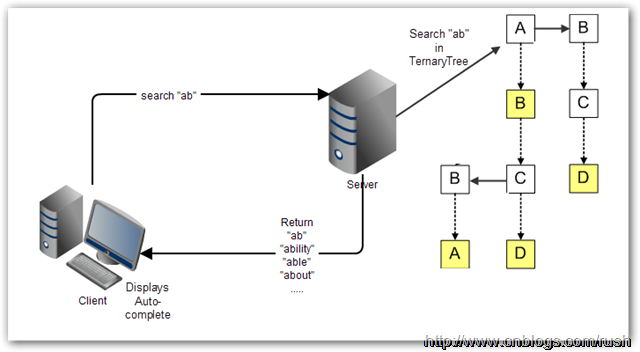
* Auto-completion: 使用搜尋引擎進行時,提供自動完成(Auto-complete)功能,讓使用者更容易查詢相關資訊
對於 Web 應用程式來說,自動完成的繁重處理工作絕大部分要交給伺服器。許多時候,自動完成不適宜一下子全都下載到客戶端,TST 是保存在伺服器上,客戶端把使用者已輸入的開頭詞彙提交到伺服器進行查詢,然後伺服器依據 TST 獲取相對應的資料列表,最後把候選的資料列表返回給客戶端。
* [Autocomplete using a ternary search tree](https://github.com/jdrnd/autocomplete-ternary)
* [Ternary Search Tree 視覺化](https://www.cs.usfca.edu/~galles/visualization/TST.html)
* 以 `ab`, `abs`, `absolute` 等字串逐次輸入並觀察
* 整合案例: [Phonebook](https://github.com/raestio/Phone_book): adds new contacts and effectively search for contacts via ternary search tree
### Trie
[trie](https://en.wikipedia.org/wiki/Trie) 與 binary search tree 不同在於,不把整個字串包在同一個節點中 ,而是根據節點的位置決定代表的字串為何。也就是一個看結果(最終節點),一個看過程 (經過的節點)。因此利用 trie 可快速找出有相同 prefix 的字串。以下舉例示範 trie 如何儲存資料。
延伸閱讀: [字典樹 Trie](http://pisces.ck.tp.edu.tw/~peng/index.php?action=showfile&file=f743c2923f8170798f62a585257fdd8436cd73b6d)
以下逐步建構 trie:
:::info
一開始,trie tree 起始於一個空的 root: ==◎==
:::
```
◎
```
:::info
先插入一個字串 `and`
1. 首先將 and 拆解成 ==a==, ==n==, ==d==
2. 因為 a 第一次出現,所以在 root 建立一個新 children node,內含值為 a
3. 接下來從 node "a" 出發,剩下 n, d
4. n 也是第一次出現,因此在 a 建立一個新 children node,內含值為 n
5. d 比照 4 作法。
:::
```
◎
/
a
/
n
/
d
```
:::info
再插入一個字串 `ant`
1. ant 拆解成 ==a==, ==n==, ==t==,從 root 出發
2. node "a" 已經存在,因此不需要自 root 創造新的 children
3. 再來看 n,node "a" 往 children 看發現 node "n" 已存在,因此也不創造 children
4. 再來看 t 發現 n 的 children 中沒有此 node,因此創造新 children "t"
:::
```
◎
/
a
/
n
/ \
d t
```
:::info
隨後插入 ==bear==
bea 會產生像這樣子的 tree
1. 有內含數值者就是有字串存在的 node
2. 因此搜尋 "ant" 會返回 0,表示 trie 內有此字串
4. 搜尋 "be" 會返回 NULL,因為在 node "e" 無有效數值
:::
```
◎
/ \
a b
/ \
n e
/ \ \
d t a (3)
(0) (1) \
r (2)
```
以上,我們注意到 trie 中,若有儲存的字串有許多相同的 prefix ,那麼 trie 可以節省大量儲存空間,考慮到 C-style string 的設計,因為 Trie 中每個字串都是經由一個字元接著另一個字元的形式來儲存,所以具有相同 prefix 的部份都會有共同的 node。
相對的,若是資料非常大量,而且幾乎沒有相同的 prefix,將會非常浪費儲存空間。因為 trie 在記憶體的儲存方式其實是像下圖這樣,每個 node 建立時,都必須同時創造 26 個值為 NULL 的子節點。
:::success
下圖的 `universal set = { a, b, c, d, e}`,所以只創造了 5 個
:::

### Ternary search tree
引入 [Ternary search tree](https://en.wikipedia.org/wiki/Ternary_search_tree) (TST),可望解決上述記體開銷的問題。這種樹的每個節點最多只會有 3 個 children,分別代表小於,等於,大於。
以下範例解釋 Ternary search tree 的運作。
:::info
插入一個字串 `and`
與 trie 概念相同,但是在 root 是直接擺 ==a==,而不需要一個 null
:::
```
a
|
n
|
d
```
:::info
接著插入單字 `ant`
1. 我們先比對 ==a==,發現 a 和 root 的字母相同(a=a)
2. 因此 pointer 往下,來到 ==n== 節點,發現 n 節點和 ant 的第二個字母相同(n=n)
3. 因此 pointer 再往下,來到 d 節點,發現 d 節點和 ant 的第三個字母不同,而且 **t > d**
4. 因此 d 節點的 right child 成為 ==t==,成功將 ant 放入原本的 TST 中
:::
```
a
|
n
|
d-
|
t
```
:::info
接著插入單字 `age`
1. 我們先比對 ==a== ,發現 a 和 root 的字母相同(a=a)
2. 因此 pointer 往下,來到 n 節點,發現 n 節點和 age 的第二個字母不同,而且 **g < n**
3. 因此 n 節點的 left child 成為 ==g==,成功將 age 放入原本的 TST 中
:::
```
a
|
-n
| |
g d-
| |
e t
```
[Ternary Search Tree ](https://www.cs.usfca.edu/~galles/visualization/TST.html) 此網址提供了透過動畫呈現,展示如何加入與刪除給定字串的流程。
我們可發現 TST 幾種特性:
1. 解決 trie tree 中大量佔用記憶體的情況,因為 TST 中,每個 node 最多只會有 3 個 child
2. 但尋找時間在某些狀況中,會比 trie 慢,這是因為 TST 插入的順序會影響比較的次數。
考慮以下兩種插入順序:
* 前者用 `aa` :arrow_right: `ac` :arrow_right: `ae` :arrow_right: `af` :arrow_right: `ag` :arrow_right: `ah` 的順序
* 後者是 `af` :arrow_right: `ae` :arrow_right: `ac` :arrow_right: `aa` :arrow_right: `ag` :arrow_right: `ah` 的順序
試想,如果我們要尋找 `ah`,那麼前者要比較 6 次,後者只要比較 3 次。而若是建立 trie ,只需要 2 次。
- [ ] 用 `aa -> ac -> ae -> af -> ag -> ah` 的順序插入

- [ ] 用 `af -> ae -> ac -> aa -> ag -> ah` 的順序插入

延伸閱讀:
* [prefix-search 報告](https://hackmd.io/s/H1ZtymjpG)
* [prefix-search 講解錄影](https://www.youtube.com/watch?v=piZ1yQH6B1I)
## [ternary search tree](https://en.wikipedia.org/wiki/Ternary_search_tree) 的實作程式碼
* 取得 [dict](https://github.com/sysprog21/dict) 程式碼,編譯並測試
```shell
$ git clone https://github.com/sysprog21/dict
$ cd dict
$ make
$ ./test_cpy
```
* 預期會得到以下執行畫面:
```
ternary_tree, loaded 259112 words in 0.151270 sec
Commands:
a add word to the tree
f find word in tree
s search words matching prefix
d delete word from the tree
q quit, freeing all data
choice:
```
* 按下 `f` 隨後按下 Enter 鍵,會得到 `find word in tree:` 的提示畫面,輸入 `Taiwan` (記得按 Enter),預期會得到以下訊息:
```
find word in tree: Taiwan
found Taiwan in 0.000002 sec.
```
* 當再次回到選單時,按下 `s` 隨後按下 Enter 鍵,會得到 `find words matching prefix (at least 1 char):` 的提示訊息,輸入 `Tain`,預期會得到以下訊息:
```
Tain - searched prefix in 0.000011 sec
suggest[0] : Tain,
suggest[1] : Tainan,
suggest[2] : Taino,
suggest[3] : Tainter
suggest[4] : Taintrux,
```
* 不難發現 prefix-search 的功能,可找出給定開頭字串對應資料庫裡頭的有效組合,你可以用 `T` 來當作輸入,可得到[世界 9 萬多個城市](https://github.com/sysprog21/dict/blob/master/cities.txt)裡頭,以 `T` 開頭的有效名稱
* 至於選單裡頭的 `a` 和 `d` 就由你去探索具體作用
## 何謂 Bloom Filter
Bloom filter 利用 hash function,在不用走訪全部元素的前提,**預測**特定字串是否存於資料結構中。因此時間複雜度是 $O(1)$,而非傳統逐一尋訪的 $O(n)$ 。
* n-bits 的 table
* k 個 hash fucntion: h~1~ 、 h~1~ ... h~k~
* 每當要加入新字串 s 時,會將 s 透過這 k 個 hash function 各自轉換為 table index (範圍: `0` 到 `n - 1`) ,所以有 k 個 hash function ,就該有 k 個 index ,然後將該 `table[index]` 上的 bit set
* 下次若要檢查該字串 s 是否存在時,只需要再跑一次那 k 個 hash function ,並檢查是否所有的 k 個 bit 都是 set 即可

* 動畫: [Cube Drone - Bloom Filters](https://www.youtube.com/watch?v=-SuTGoFYjZs)
但這做法**存在錯誤率**,例如原本沒有在資料結構中的字串 s1 經過 hash 轉換後得出的 bit 的位置和另一個存在於資料結構中的字串 s2 經過 hash 之後的結果相同,如此一來,先前不存在的 s1 便會被認為存在,這就是 [false positive](https://en.wikipedia.org/wiki/False_positives_and_false_negatives) (指進行實用測試後,測試結果有機會不能反映出真正的面貌或狀況)。
Bloom filter 一類手法的應用很常見。例如在社群網站 Facebook,在搜尋欄鍵入名字時,能夠在 [20 億個註冊使用者](https://www.bnext.com.tw/article/45104/facebook-maus-surpasses-2-billion) (2017 年統計資料) 中很快的找到結果,甚至是根據與使用者的關聯度排序。
延伸閱讀:
* [Esoteric Data Structures and Where to Find Them](https://youtu.be/-8UZhDjgeZU?t=607)
* [Bloom Filter 影片解說](https://www.youtube.com/watch?v=bEmBh1HtYrw)
- [ ] Bloom Filter 實作方式
首先,建立一個 n bits 的 table,並將每個 bit 初始化為 0。
我們將所有的字串構成的集合 (set) 表示為 S = { x~1~, x~2~, x~3~, ... ,x~n~ },Bloom Filter 會使用 k 個不同的 hash function,每個 hash function 轉換後的範圍都是 0 到 n-1 (為了能夠對應上面建立的 n bits table)。而對每個 S 內的 element x~i~,都需要經過 k 個 hash function,一一轉換成 k 個 index。轉換過後,table 上的這 k 個 index 的值就必須設定為 `1`。
> 注意: 可能會有同一個 index 被多次設定為 `1` 的狀況
Bloom Filter 這樣的機制,存在一定的錯誤率。若今天想要找一個字串 x 在不在 S 中,這樣的資料結構只能保證某個 x~1~ 一定不在 S 中,但沒辦法 100% 確定某個 x~2~一定在 S 中。因為會有誤判 (false positive ) 的可能。
此外,資料只能夠新增,而不能夠刪除,試想今天有兩個字串 x~1~, x~2~ 經過某個 hash function h~i~ 轉換後的結果 h~i~(x~1~) = h~i~(x~2~),若今天要刪除 x~1~ 而把 table 中 set 的 1 改為 0,豈不是連 x~2~ 都受到影響?
- [ ] Bloom Filter 錯誤率計算
首先假設我們的所有字串集合 S 裡面有 n 個字串, hash 總共有 k 個,Bloom Filter 的 table 總共 m bits。我們會判斷一個字串存在於 S 內,是看經過轉換後的每個 bits 都被 set 了,我們就會說可能這個字串在 S 內。但試想若是其實這個字串不在 S 內,但是其他的 a b c 等等字串經過轉換後的 index ,剛好涵蓋了我們的目標字串轉換後的 index,就造成了誤判這個字串在 S 內的情況。
如上述,Bloom Filter 存有錯誤機率,程式開發應顧及回報錯誤機率給使用者,以下分析錯誤率。
當我們把 S 內的所有字串,每一個由 k 個 hash 轉換成 index 並把 `table[index]` 設為 1,而全部轉完後, table 中某個 bits 仍然是 0 的機率是 $(1-\dfrac{1}{m})^{kn}$ 。
其中 $(1-\dfrac{1}{m})$ 是每次 hash 轉換後,table 的某個 bit 仍然是 0 的機率。因為我們把 hash 轉換後到每個 index (而這個 index 會被 set) 的機率視為相等 (每人 $\dfrac{1}{m}$),所以用 1 減掉即為不會被 set 的機率。我們總共需要做 kn 次 hash,所以就得到答案$(1-\dfrac{1}{m})^{kn}$。
由 $(1-\dfrac{1}{m})^{m}≈e^{-1}$ 特性,$(1-\dfrac{1}{m})^{kn}=((1-\dfrac{1}{m})^{m})^{\frac{kn}{m}}≈(e^{-1})^{\frac{kn}{m}}≈e^{-\frac{kn}{m}}$
以上為全部的字串轉完後某個 bit 還沒有被 set 的機率。
因此誤判的機率等同於全部經由 k 個 hash 轉完後的 k bit 已經被其他人 set 的機率:
轉完後某個 bit 被 set 機率是: $1-e^{-\frac{kn}{m}}$,因此某 k bit 被 set 機率為: ==$(1-e^{-\frac{kn}{m}})^k$==
延伸閱讀:
* [Bloom Filter](https://blog.csdn.net/jiaomeng/article/details/1495500)
### 如何選參數值
* k: 多少個不同 hash
* m: table size 的大小
**如何選 k 值?**
我們必須讓錯誤率是最小值,因此必須讓 $(1-e^{-\frac{kn}{m}})^k$ 的值是最小。先把原式改寫成 $(e^{k\ ln(1-e^{-\frac{kn}{m}})})$,我們只要使 ${k\ ln(1-e^{-\frac{kn}{m}})}$ 最小,原式就是最小值。可以看出當 $e^{-\frac{kn}{m}}=\dfrac{1}{2}$ 時,會達到最小值。因此 ==$k=ln2\dfrac{m}{n}$== 即能達到最小值。
[Bloom Filter calculator](https://hur.st/bloomfilter/?n=5000&p=3&m=&k=45) 和 [Bloom Filter calculator 2](https://krisives.github.io/bloom-calculator/) 這兩個網站可以透過設定自己要的錯誤率與資料的多寡,得到 `k` 和 `m` 值。
## 在 prefix search 導入 Bloom filter 機制
[參考的字典檔案](https://stackoverflow.com/questions/4456446/dictionary-text-file) 裡面總共有 36922 個詞彙。
經由上述運算得知,當我們容許 5% 錯誤 (=0.05) 時:
* table size = 230217
* k = 4
先用原來的 `cities.txt` 檔案做測試,以驗證估程式。
首先,這裡選用了兩種 hash function:`jenkins` 和`djb2`,另外 [murmur3 hash](https://en.wikipedia.org/wiki/MurmurHash) 也是個不錯的選擇,這裡主要是選用夠 uniform 的即可。
```cpp
unsigned int djb2(const void *_str) {
const char *str = _str;
unsigned int hash = 5381;
char c;
while ((c = *str++))
hash = ((hash << 5) + hash) + c;
return hash;
}
unsigned int jenkins(const void *_str) {
const char *key = _str;
unsigned int hash=0;
while (*key) {
hash += *key;
hash += (hash << 10);
hash ^= (hash >> 6);
key++;
}
hash += (hash << 3);
hash ^= (hash >> 11);
hash += (hash << 15);
return hash;
}
```
再來宣告我們的 Bloom filter 主體,這裡用一個結構體涵蓋以下:
* `func` 是用來把我們的 hash function 做成一個 list 串起來,使用這個方法的用意是方便擴充。若我們今天要加進第三個 hash function,只要串進 list ,後面在實做時就會走訪 list 內的所有 function。
* `bits` 是我們的 filter 主體,也就是 table 。 size 則是 table 的大小。
```cpp
typedef unsigned int (*hash_function)(const void *data);
typedef struct bloom_filter *bloom_t;
struct bloom_hash {
hash_function func;
struct bloom_hash *next;
};
struct bloom_filter {
struct bloom_hash *func;
void *bits;
size_t size;
};
```
主要的程式碼如下。
首先在 `bloom_create` 的部份,可以看到我們把兩個 hash function 透過`bloom_add_hash` 加入結構中。
再來 `bloom_add` 裡面是透過對目標字串 `item` 套用 hash ,並把 hash 產生的結果對 `filter->size` 取餘數 (第 19 行),這樣才會符合 table size 。最後第 19 行把產生的 bit 設定為 1 。
最後`bloom_test`就是去檢驗使用者輸入的 `item` 是不是在結構當中。與 add大致上都相等,只是把 bit 設定為 1 的部份改為「檢驗是不是 1」,若是任一個 bit 不是 1 ,我們就可以說這個結構裡面沒有這個字串。
這樣的實做,讓我們可以在 bloom_create 初始化完,接下來要加入字串就呼叫 bloom_add ,要檢驗字串就呼叫 bloom_test,不需要其他的操作。
```cpp=
bloom_t bloom_create(size_t size) {
bloom_t res = calloc(1, sizeof(struct bloom_filter));
res->size = size;
res->bits = malloc(size);
// 加入 hash function
bloom_add_hash(res, djb2);
bloom_add_hash(res, jenkins);
return res;
}
void bloom_add(bloom_t filter, const void *item) {
struct bloom_hash *h = filter->func;
uint8_t *bits = filter->bits;
while (h) {
unsigned int hash = h->func(item);
hash %= filter->size;
bits[hash] = 1;
h = h->next;
}
}
bool bloom_test(bloom_t filter, const void *item) {
struct bloom_hash *h = filter->func;
uint8_t *bits = filter->bits;
while (h) {
unsigned int hash = h->func(item);
hash %= filter->size;
if (!(bits[hash])) {
return false;
}
h = h->next;
}
return true;
}
```
再來是 `main` 改的部份,這裡修改 `test_ref.c` 檔案。需要更動的地方是 add 和 find 功能 (delete 會失去效用,注意!)
首先 find 功能修改:
```cpp=
t1 = tvgetf();
// 用 bloom filter 判斷是否在 tree 內
if (bloom_test(bloom, word) == 1) {
// version1: bloom filter 偵測到在裡面就不走下去
t2 = tvgetf();
printf(" Bloomfilter found %s in %.6f sec.\n", word, t2 - t1);
printf(" Probability of false positives:%lf\n", pow(1 - exp(-(double)HashNumber / (double) ((double) TableSize /(double) idx)), HashNumber));
// version2: loom filter 偵測到在裡面,就去走 tree (防止偵測錯誤)
t1 = tvgetf();
res = tst_search(root, word);
t2 = tvgetf();
if (res)
printf(" ----------\n Tree found %s in %.6f sec.\n", (char *) res, t2 - t1);
else
printf(" ----------\n %s not found by tree.\n", word);
} else
printf(" %s not found by bloom filter.\n", word);
break;
```
由以上可見,第 3 行會先用 bloom filter 去判斷是否在結構內,若不存在的話就不用走訪。如果在的話,程式印出 bloom filter 找到的時間,以及錯誤機率,隨後走訪節點,判斷是否在 tree 裡面。
上述參數的配置為:
* TableSize = 5000000 (=五百萬)
* hashNumber = 2 (總共兩個 hash)
* 用原來的 `cities.txt` 數據量為 259112
計算出理論錯誤率約為 `0.009693`,也就是不到 `1%`。
以下是 add 的部份:
```clike=
if (bloom_test(bloom, Top) == 1) // 已被 Bloom filter 偵測存在,不要走 tree
res = NULL;
else { // 否則就走訪 tree,並加入 bloom filter
bloom_add(bloom,Top);
res = tst_ins_del(&root, &p, INS, REF);
}
t2 = tvgetf();
if (res) {
idx++;
Top += (strlen(Top) + 1);
printf(" %s - inserted in %.10f sec. (%d words in tree)\n",(char *) res, t2 - t1, idx);
} else
printf(" %s - already exists in list.\n", (char *) res);
if (argc > 1 && strcmp(argv[1], "--bench") == 0) // a for auto
goto quit;
break;
```
以上程式碼可以看到,第 1 行的部份會先偵測要加入的字串是否在結構中,若是回傳 1 表示 bloom filter 偵測在結構中,已經重複了。因此會把 res 設為 null,這樣下方第 9 行的判斷自然就不會成立。如果偵測字串不在結構中,會跑進第 3 行的 else,加入結構還有 Bloom filter 當中。
### 分飾多角的 eqkid
資料結構:
```cpp
typedef struct tst_node {
char key; /* char key for node (null for node with string) */
unsigned refcnt; /* refcnt tracks occurrence of word (for delete) */
struct tst_node *lokid; /* ternary low child pointer */
struct tst_node *eqkid; /* ternary equal child pointer */ /** 其實它分飾多角 **/
struct tst_node *hikid; /* ternary high child pointer */
} tst_node;
```
`tst_ins_del` 實作:
```cpp
void *tst_ins_del(tst_node **root, const char *s, const int del, const int cpy)
{
...
while ((curr = *pcurr)) { /* iterate to insertion node */
...
return (void *) curr->eqkid; /* pointer to word */
...
pcurr = &(curr->eqkid); /* get next eqkid pointer address */
...
}
for (;;) {
...
curr->eqkid = (tst_node *) s;
return (void *) s;
...
}
}
```
乍看之下一頭霧水,為何有時將 `eqkid` 傳出去當 word 起始位置,有時又用它來取得下個 node,有時將傳進來的 `const char *s` 轉型成 `tst_node *` 呢?其實從 `tst_suggest` 可以看出些端倪:
```cpp
void tst_suggest( ... )
{
...
if (p->key)
tst_suggest(p->eqkid, c, nchr, a, n, max);
else if (*(((char *) p->eqkid) + nchr - 1) == c)
a[(*n)++] = (char *) p->eqkid;
...
}
```
若 `key` 非 0(`key` 爲 0 的 node 的存在是爲了表示 parent node 的結尾),則將 `eqkid` 當 node 指標進行 recursive call,否則當作字串使用。
這裡需要記錄字串是因爲走訪到 node 之後要得知該 node 代表的字串是有點麻煩的事情(若有記錄 parent,可以往上透過一些規則找回),但這裡很巧妙的利用了 `eqkid` 當作 `char *` 指向該 node 表示的字串。
關於程式碼的 copy (`CPY`) 與 reference (`REF`) 機制,前者是傳入 `tst_ins_del` 的字串地址所表示的值**隨時會被覆寫**,因此 `eqkid` 需要 `malloc` 新空間將其 **copy** 存起來,而後者是傳進來的字串地址所表示的值**一直屬於該字串**,以此可將其當作 **reference** 直接存起來,不用 `malloc` 新空間。
承接上面,`eqkid` 分飾多角,沒有需要重複使用的時候嗎?
|Insert XY|Insert XYZ|Insert XY and XYZ
|--|--|--|
|  |  |  |
如上面第三種情況,node Z 的 `eqkid` 該指向 ``"XY"`` 表示該字串結束,還是指向下一個 `key` 爲 0 的 node 表示 `"XYZ"` 的結束呢?
再仔細觀察及思考會發現 node Z 的 key 爲 `'z'`,已無法表示字串 `"XY"` 的結束,`tst_node` 中也沒有類似綠色的屬性,所以 tst.c 的實作實際上是這樣的:
|Insert XY and XYZ in order|Insert XYZ and XY in order|
|--|--|
|||
> 注意:上圖(兩張都)請將 N 當作小綠空圓(表示字串 `"XY"` 的結束)並無視它下面的小綠空圓,而左圖 `>N` 爲 `>0`
可見用來表示結束的 node 永遠不會有 ternary equal child, 因此 `eqkid` 就不會分身乏術。
## 透過統計模型來分析資料
[dict](https://github.com/sysprog21/dict) 程式碼中的 copy 與 reference 機制:
* copy 機制 (`CPY`): 傳入 `tst_ins_del` 的字串地址所表示的值**隨時會被覆寫**,因此 `eqkid` 需要 `malloc` 新空間將其 **copy** 存起來;
* reference 機制 (`REF`): 傳進來的字串地址所表示的值**一直屬於該字串**,以此可將其當作 **reference** 直接存起來,不用透過 `malloc` 新空間。
參照交通大學開放課程: [統計學(一)](http://ocw.nctu.edu.tw/course_detail.php?bgid=3&gid=0&nid=277) / [統計學(二)](http://ocw.nctu.edu.tw/course_detail.php?bgid=3&gid=0&nid=511)
* 95% 信賴區間是從樣本數據計算出來的一個區間,在鐘形曲線的條件下,由樣本回推,「可能」會有 95 % 的機會把真正的母體參數包含在區間之中
* 鐘形曲線可見資料的密集與散佈與否
* 圖形上第一個數為平均,第二個數為標準差的平方,我們稱以下圖形為機率密度函數 Probability Density Function (PDF)

* 雖然不一定每種統計數據都是常態分佈,但只要資料是常態分佈,機率密度函數就會成鐘形曲線,這是我們所希望的,因為排除掉忽大忽小的個案,才可以掌握資訊的正確性
把 [dict](https://github.com/sysprog21/dict) 程式碼和給定的資料分用從 CPY 和 REF,用統計的方式重畫,其中 X-axis 是 cycles 數,Y-axis 是到目前為止已累積多少筆相同 cycle 數的資料。
- [ ] CPY 分析分佈

- [ ] REF (+Memory pool) 分析分佈

轉換圖表 X-Y 的數據後我們可以很明顯的看出 REF 資料密集程度遠大於 CPY ,不只在 count 累積的數目,也在 cycles 的 range 有很大的差異
* 計算平均與標準差:
標準差 $\sigma=\sqrt{\dfrac{1}{N}\cdot\sum_{k=1}^{N}(X_i-\overline{x})^2}$
* CPY 平均: 5974.116 cycles
* CPY 標準差: 5908.070
* REF 平均: 65.885 cycles
* REF 標準差: 9.854
* 帶入機率密度函數公式:
$f(x) = {1 \over \sigma\sqrt{2\pi} }\,e^{- {{(x-\mu )^2 \over 2\sigma^2}}}$
* 把 x 帶入後,在常態分佈下資料展現如下圖。要特別注意是,因為我們判定資料型態像常態分佈才用這個公式算出理想的模型,CPY 表現太分散,其實並不像常態分佈所以才會在算 95% 信賴區間(平均加減 2 倍標準差)時出現負數,而 REF 符合常態分佈,在此假設他們是常態分佈下才能做以下的鐘形曲線圖
* probability 總和為 1,因為資料量大,所以如果愈分散每個 cycles 分到的機率愈小
- [ ] REF_PDF ideal model (理想情況):

- [ ] REF_PDF real model (真實情況):

顯然真實情況偏離理想狀況,但我們可將出現機率很小且不符合 95% 信賴區間的數值拿掉不考量。
- [ ] CPY_PDF real model

* CPY 除了非常不符合常態分佈以外,還有個更糟糕的情況,我們出現機率少的數值竟然佔大多數,可見資料是十分分散的,所以這邊我們不能取 95% 信賴間,因此得重新分析 CPY_PDF。
- [ ] Poisson distribution
參考 [Statistics The Poisson Distribution ](https://www.umass.edu/wsp/resources/poisson/), [統計應用小小傳](http://www.agron.ntu.edu.tw/biostat/Poisson.html) , [Wikipedia](https://en.wikipedia.org/wiki/Poisson_distribution)
> The fundamental trait of the Poisson is its asymmetry, and this trait it preserves at any value of ${\lambda }$
有別於我們一般常態分佈的對稱性,不對稱性剛好是 Poisson 分布的特色

x 軸代的 k 是 indexm, y 軸則是代入 k 後的機率
* Probability of events for a Poisson distribution:
P ( k events in interval ) = $e^{-\lambda}\cdot\dfrac{{\lambda}^k}{k!}$
* 只需要一個參數 : 單位時間平均事件發生次數 λ
* 要判定一個統計是否可以做出 Poisson distribution 必須要有以下特點:
1. the event is something that can be counted in whole numbers
2. occurrences are independent
3. the average frequency of occurrence for the time period is known
4. it is possible to count how many events have occurred
$\lambda$ 代 $\frac{1}{\mu}$ : 這邊的意思拿 CPY 來說就是平均每 5974.116 個 cycle 可以完成一次搜尋。但為了做圖方便所以將 5974.116 (cycles) 為一個單位時間,這樣 $\lambda$ 代 1

放大版本

ideal 為階梯狀的原因是 5974.116 cycles 為一個單位,然後公式裏面又有 k 階層,所以在小數的部份會被忽略,但 real 的部份又是 1 個 cycle 為單位,應以 5974.116 cycles 為單位製圖較容易觀察差異。
以 5974.116 cycles 為一個單位製圖

* 代入 Poisson 的 95% confidence interval
* 參考 [How to calculate a confidence level for a Poisson distribution?](https://stats.stackexchange.com/questions/15371/how-to-calculate-a-confidence-level-for-a-poisson-distribution)
* 兩者的 95% 信賴區間
* CPY = 5477.26 ~ 6947.76 (cycles)
* REF (+memory pool) = 46.177 ~ 85.593 (cycles)
## 使用 perf 分析程式效能
參考 [使用 perf_events 分析程式效能](https://zh-blog.logan.tw/2019/07/10/analyze-program-performance-with-perf-events/) 和 [簡介 perf_events 與 Call Graph](https://zh-blog.logan.tw/2019/10/06/intro-to-perf-events-and-call-graph/) 這兩份中文介紹。
在 `Makefile` 新增 `perf-search` 標的:
```shell
perf-search: $(TESTS)
@for test in $(TESTS); do\
echo 3 | sudo tee /proc/sys/vm/drop_caches; \
perf stat \
-e cache-misses,cache-references,instructions,cycles \
./$$test --bench; \
done
```
執行 `make perf-search`
```shell
Performance counter stats for './test_cpy --bench':
1,681,368,653 cache-misses # 58.179 % of all cache refs
2,890,009,712 cache-references 49,637,166,894 instructions # 0.90 insn per cycle
54,932,228,832 cycles 15.492978290 seconds time elapsed
Performance counter stats for './test_ref --bench':
1,967,405,626 cache-misses # 62.223 % of all cache refs
3,161,862,019 cache-references 49,705,117,369 instructions # 0.71 insn per cycle
70,053,549,114 cycles 19.957402867 seconds time elapsed
```
明明搜索過程一致,但兩者的 cache-misses 次數卻相差甚遠。
仔細思考兩者的差異,其實**只有** ternimal node 的 `eqkid` 所指向的**字串地址來源不同**,CPY 機制是單獨 `malloc` 的小空間,REF 機制是 `malloc` 大空間的一小部分。所以過程中的差異是,僅最後對字串地址進行 dereference,到對應的地址讀出字串的地方。
嘗試刪掉最後的 dereference 相關的部分(原本用來檢查是否找到符合的 prefix,刪掉會導致結果不正確,但這裡的重點是尋找 REF 相對耗時的地方:
```cpp
void tst_suggest(const tst_node *p,
const char c,
const size_t nchr,
char **a,
int *n,
const int max)
{
if (!p || *n == max)
return;
tst_suggest(p->lokid, c, nchr, a, n, max);
if (p->key)
tst_suggest(p->eqkid, c, nchr, a, n, max);
else // if (*(((char *) p->eqkid) + nchr - 1) == c) <= delete this only
a[(*n)++] = (char *) p->eqkid;
tst_suggest(p->hikid, c, nchr, a, n, max);
}
```
重新用 perf 分析:
```
Performance counter stats for './test_cpy --bench':
1,390,728,865 cache-misses # 52.515 % of all cache refs
2,648,254,194 cache-references 45,808,349,880 instructions # 0.97 insn per cycle
47,022,265,491 cycles 12.974203801 seconds time elapsed
Performance counter stats for './test_ref --bench':
1,340,926,158 cache-misses # 50.404 % of all cache refs
2,660,373,578 cache-references 45,869,337,319 instructions # 0.98 insn per cycle
46,894,627,000 cycles 12.866257905 seconds time elapsed
```

也就是說,造成 REF 相對慢的原因,與 `*(((char *) p->eqkid) + nchr - 1)` 操作有關。
進一步用 perf 分析每個 intruction 發生 cache miss 的次數:
```shell
$ perf record -e cache-misses ./test_ref --bench && perf report`
98.89% test_ref test_ref [.] tst_suggest
0.22% test_ref test_ref [.] tst_search_prefix
0.08% test_ref test_ref [.] tst_ins_del
```
由於測試的是 prefix-search,時間都花在 `tst_suggest` 上不意外,先附上 [`tst_suggest`]() 前半段中每一行程式碼對應的組語指令
```cpp
tst_suggest():
const tst_node *p, // -0x8 相對於 %rbp 的地址
const char c, // -0xc
const size_t nchr, // -0x18
char **a, // -0x20
int *n, // -0x28
const int max) // -0x10
{
push %rbp
mov %rsp,%rbp
sub $0x30,%rsp
mov %rdi,-0x8(%rbp)
mov %esi,%eax
mov %rdx,-0x18(%rbp)
mov %rcx,-0x20(%rbp)
mov %r8,-0x28(%rbp)
mov %r9d,-0x10(%rbp)
mov %al,-0xc(%rbp)
if (!p || *n == max)
cmpq $0x0,-0x8(%rbp)
↓ je 10e
mov -0x28(%rbp),%rax
mov (%rax),%eax
cmp %eax,-0x10(%rbp)
↓ je 10e
return;
tst_suggest(p->lokid, c, nchr, a, n, max);
movsbl -0xc(%rbp),%esi
mov -0x8(%rbp),%rax
mov 0x8(%rax),%rax
mov -0x10(%rbp),%r8d
mov -0x28(%rbp),%rdi
mov -0x20(%rbp),%rcx
mov -0x18(%rbp),%rdx
mov %r8d,%r9d
mov %rdi,%r8
mov %rax,%rdi
→ callq tst_suggest
if (p->key)
mov -0x8(%rbp),%rax
movzbl (%rax),%eax
test %al,%al
↓ je 9c
tst_suggest(p->eqkid, c, nchr, a, n, max);
movsbl -0xc(%rbp),%esi
mov -0x8(%rbp),%rax
mov 0x10(%rax),%rax
mov -0x10(%rbp),%r8d
mov -0x28(%rbp),%rdi
mov -0x20(%rbp),%rcx
mov -0x18(%rbp),%rdx
mov %r8d,%r9d
mov %rdi,%r8
mov %rax,%rdi
→ callq tst_suggest
↓ jmp e2
else if (*(((char *) p->eqkid) + nchr - 1) == c)
9c: mov -0x8(%rbp),%rax
mov 0x10(%rax),%rax
mov -0x18(%rbp),%rdx
sub $0x1,%rdx
add %rdx,%rax
movzbl (%rax),%eax
cmp %al,-0xc(%rbp)
↓ jne e2
a[(*n)++] = (char *) p->eqkid;
mov -0x28(%rbp),%rax
...
10e: nop
}
```
儘管上方為 x86_64 組合語言,但我們只需要理解 `mov` 時 `0x8(%rax)` 會對 `%rax + 0x8` 這地址做 dereference,而 `(%rax)` 可理解爲 `0x0(%rax)` 的縮寫。
另外還需知道 [x86 General registers ](http://www.eecg.toronto.edu/~amza/www.mindsec.com/files/x86regs.html)。
```
32 bits : EAX EBX ECX EDX
16 bits : AX BX CX DX
8 bits : AH AL BH BL CH CL DH DL
```
進一步比較兩種機制的差異,左邊的數值是 cache miss 發生在該指令的 period。
- [ ] `test_ref`
2 處熱點:

和

- [ ] `test_cpy`
1 處熱點


爲什麼第一處是發生在 `mov -0x10(%rbp),%r8d`(把 `max` 的值給 `%r8d` register),原來 [perf 在回報時會有偏差](https://stackoverflow.com/questions/43794510/linux-perf-reporting-cache-misses-for-unexpected-instruction),於是這裡看似實際發生 cache miss 是在上一個 instruction:
`mov 0x8(%rax),%rax`
即對 p 做 dereference(這裡是 function 裡的第一次,之後這 function 再對 `p` 做 dereference 時就很大機率 cache hit)
`p->lokid` =>`(*p).lokid`
其實以編譯器的角度(也是實際過程)應該是
`*(tst_node*)((char*)p + offsetof(tst_node, lokid))`
這裡的 `0x8` 即是所謂的 `offsetof(tst_node, lokid)`(在編譯時期可算出,對應指令中的 `0x8`),`rax` 在這裡是 `p`。
第二處便是之前提到的字串 dereference
`*(((char *) p->eqkid) + nchr - 1)`
這裡一樣有回報偏差,實際上也是上一道指令 `movzbl (%rax),%eax`),原先推測 REF 機制在這裡發生 cache miss 的機率只是比 CPY 機制稍高,沒想到竟然高了**十幾倍**!應該說 CPY 機制在這裡完全沒有特別容易 cache miss 的傾向。
把地址印出觀察:
```cpp
void tst_suggest (...)
{
...
if (p->key)
tst_suggest(p->eqkid, c, nchr, a, n, max);
else {
if (*(((char *) p->eqkid) + nchr - 1) == c)
a[(*n)++] = (char *) p->eqkid;
printf("%p\n", (((char *) p->eqkid) + nchr - 1));
}
...
}
```
測試:
```shell
# ./test_cpy --bench`:
0x556d88e35022
0x556d88d31862
0x556d88cedf92
0x556d8870d522
...
# ./test_ref --bench`:
0x7f76374d48d7
0x7f763735fcf8
0x7f76374b9321
0x7f763743ac33
...
```
回頭看 [malloc 的描述](https://linux.die.net/man/3/malloc):
> **NOTES**
Normally, malloc() allocates memory from the heap, and adjusts the size of the heap as required, using sbrk(2). When allocating blocks of memory larger than MMAP_THRESHOLD bytes, the glibc malloc() implementation allocates the memory as a private anonymous mapping using mmap(2). MMAP_THRESHOLD is 128 kB by default, but is adjustable using mallopt(3). Prior to Linux 4.7 allocations performed using mmap(2) were unaffected by the RLIMIT_DATA resource limit; since Linux 4.7, this limit is also enforced for allocations performed using mmap(2).
原來在 GNU/Linux 中,`malloc` 面對大於 `MMAP_THRESHOLD` bytes 的空間時,會呼叫 `mmap`,而 `mmap` 會(在 heap 和 stack 之間)建立一個 `vm_area_struct`,將檔案映射到虛擬記憶體空間。

[圖片來源](https://jin-yang.github.io/post/kernel-memory-mmap-introduce.html)
Standard segment layout in a Linux process. (32-bit)

> [圖片來源](https://manybutfinite.com/post/anatomy-of-a-program-in-memory/)
但這樣仍無法解釋實驗結果的差異,再對程式進行以下觀察:
```cpp
#include <stdint.h>
void tst_suggest (...)
{
...
if (p->key)
tst_suggest(p->eqkid, c, nchr, a, n, max);
else {
if (*(((char *) p->eqkid) + nchr - 1) == c)
a[(*n)++] = (char *) p->eqkid;
printf("%ld\n", (intptr_t)(void*)(((char *) p->eqkid) + nchr - 1) - (intptr_t)(void*)&p->lokid);
}
...
}
```
測試:
```shell
# ./test_ref --bench
45833574649567
45833579989413
45833586770473
45833588397029
...
# ./test_cpy --bench
42
42
42
42
...
```
終於找到 CPY 機制在 prefix-search 時效率比較好的原因
回想 tst.c 的 `tst_ins_del`:
```cpp
void *tst_ins_del(tst_node **root, const char *s, const int del, const int cpy)
{
...
if (*p++ == 0) {
if (cpy) { /* allocate storage for 's' */
const char *eqdata = strdup(s);
if (!eqdata)
return NULL;
curr->eqkid = (tst_node *) eqdata;
return (void *) eqdata;
} else { /* save pointer to 's' (allocated elsewhere) */
curr->eqkid = (tst_node *) s;
return (void *) s;
}
}
...
}
```
CPY 機制在 insert 時,建立 leaf 後會間接呼叫 `malloc` 來保存字串,在這之前的最後一次 `malloc` 是爲了配置該 leaf 的空間。一直 `malloc` 時,heap 也會形同 stack 一般地增長,所以像給定測試條件很規律的狀況下,字串地址與 leaf 的地址很可能都很靠近。
換言之,CPY 機制在一開始 `mov 0x8(%rax),%rax` (`p->eqkid`)後,字串就很大可能在 cache 裡面了,因此 cache miss 機率較低,這就是它相對來說在 prefix-search 上效率比較好的原因!
CPY 機制與 REF 機制在建 tree 的效率比較
+ CPY 機制
+ 讀檔時每次將地名暫時存入同一字串 `word`
:+1: 只要 cache 沒被覆蓋就不會發生 cache miss
+ ternary search tree 的 terminal node 用 `strdup` 將地名存起來
:-1: 需要複製字串(影響小)
:-1: 間接呼叫 `malloc`,可能涉及大量系統呼叫
+ REF 機制
+ 讀檔時每次將地名永久(直到 memory pool 被 free)依序存入 memory pool
:-1: cache miss 次數 $\ge$ 使用的 memory pool 大小 / cache 一次載入的大小
+ ternary search tree 的 terminal node 直接存 reference(指向 memory pool 的某個位置)
:+1: 沒有明顯額外 overhead