LUMI Training Warsaw

# LUMI Training Warsaw ### Login to Lumi ``` ssh USERNAME@lumi.csc.fi ``` To simplify the login to LUMI, you can add the following to your `.ssh/config` file. ``` # LUMI Host lumi User <USERNAME> Hostname lumi.csc.fi IdentityFile <HOME_DIRECTORY>/.ssh/id_rsa ServerAliveInterval 600 ServerAliveCountMax 30 ``` The `ServerAlive*` lines in the config file may be added to avoid timeouts when idle. Now you can shorten your login command to the following. ``` ssh lumi ``` If you are able to log in with the ssh command, you should be able to use the secure copy command to transfer files. For example, you can copy the presentation slides from lumi to view them. ``` scp lumi:/project/project_465000828/Slides/AMD/<file_name> <local_filename> ``` You can also copy all the slides with the . From your local system: ``` mkdir slides scp -r lumi:/project/project_465000828/Slides/AMD/* slides ``` If you don't have the additions to the config file, you would need a longer command: ``` mkdir slides scp -r -i <HOME_DIRECTORY>/.ssh/<public ssh key file> <username>@lumi.csc.fi:/project/project_465000828/slides/AMD/ slides ``` or for a single file ``` scp -i <HOME_DIRECTORY>/.ssh/<public ssh key file> <username>@lumi.csc.fi:/project/project_465000644/slides/AMD/<file_name> <local_filename> ``` ## HIP Exercises We assume that you have already allocated resources with `salloc` `cp -r /project/project_465000644/Exercises/AMD/HPCTrainingExamples/ .` `salloc -N 1 -p small-g --gpus=1 -t 10:00 -A project_465000644` ``` module load craype-accel-amd-gfx90a module load PrgEnv-amd module load rocm ``` The examples are also available on github: ``` git clone https://github.com/amd/HPCTrainingExamples ``` However, we recommend using the version in `/project/project_465000644/Exercises/AMD/HPCTrainingExamples` as it has been tuned to the current LUMI environment. ### Basic examples `cd HPCTrainingExamples/HIP/vectorAdd ` Examine files here – README, Makefile and vectoradd_hip.cpp Notice that Makefile requires HIP_PATH to be set. Check with module show rocm or echo $HIP_PATH Also, the Makefile builds and runs the code. We’ll do the steps separately. Check also the HIPFLAGS in the Makefile. ``` make vectoradd_hip.exe srun -n 1 ./vectoradd_hip.exe ``` We can use SLURM submission script, let's call it `hip_batch.sh`: ``` #!/bin/bash #SBATCH -p small-g #SBATCH -N 1 #SBATCH --gpus=1 #SBATCH -t 10:00 #SBATCH -A project_465000644 module load craype-accel-amd-gfx90a module load rocm cd $PWD/HPCTrainingExamples/HIP/vectorAdd export HCC_AMDGPU_TARGET=gfx90a make vectoradd srun -n 1 --gpus 1 ./vectoradd ``` Submit the script `sbatch hip_batch.sh` Check for output in `slurm-<job-id>.out` or error in `slurm-<job-id>.err` Compile and run with Cray compiler ``` CC -x hip vectoradd.hip -o vectoradd srun -n 1 --gpus 1 ./vectoradd ``` Now let’s try the cuda-stream example from `https://github.com/ROCm-Developer-Tools/HIP-Examples`. This example is from the original McCalpin code as ported to CUDA by Nvidia. This version has been ported to use HIP. See add4 for another similar stream example. ``` export HCC_AMDGPU_TARGET=gfx90a cd HIP-Examples/cuda-stream make srun -n 1 ./stream ``` Note that it builds with the hipcc compiler. You should get a report of the Copy, Scale, Add, and Triad cases. The variable `export HCC_AMDGPU_TARGET=gfx90a` is not needed in case one sets the target GPU for MI250x as part of the compiler flags as `--offload-arch=gfx90a`. Now check the other examples in `HPCTrainingExamples/HIP` like jacobi etc. ## Hipify We’ll use the same HPCTrainingExamples that were downloaded for the first exercise. Get a node allocation. ``` salloc -N 1 --ntasks=1 --gpus=1 -p small-g -A project_465000644 –-t 00:10:00` ``` A batch version of the example is also shown. ### Hipify Examples #### Exercise 1: Manual code conversion from CUDA to HIP (10 min) Choose one or more of the CUDA samples in `HPCTrainingExamples/HIPIFY/mini-nbody/cuda` directory. Manually convert it to HIP. Tip: for example, the cudaMalloc will be called hipMalloc. Some code suggestions include `nbody-block.cu, nbody-orig.cu, nbody-soa.cu` You’ll want to compile on the node you’ve been allocated so that hipcc will choose the correct GPU architecture. #### Exercise 2: Code conversion from CUDA to HIP using HIPify tools (10 min) Use the `hipify-perl` script to “hipify” the CUDA samples you used to manually convert to HIP in Exercise 1. hipify-perl is in `$ROCM_PATH/bin` directory and should be in your path. First test the conversion to see what will be converted ``` hipify-perl -no-output -print-stats nbody-orig.cu ``` You'll see the statistics of HIP APIs that will be generated. ``` [HIPIFY] info: file 'nbody-orig.cu' statisitics: CONVERTED refs count: 10 TOTAL lines of code: 91 WARNINGS: 0 [HIPIFY] info: CONVERTED refs by names: cudaFree => hipFree: 1 cudaMalloc => hipMalloc: 1 cudaMemcpy => hipMemcpy: 2 cudaMemcpyDeviceToHost => hipMemcpyDeviceToHost: 1 cudaMemcpyHostToDevice => hipMemcpyHostToDevice: 1 ``` `hipify-perl` is in `$ROCM_PATH/bin` directory and should be in your path. In some versions of ROCm, the script is called `hipify-perl`. Now let's actually do the conversion. ``` hipify-perl nbody-orig.cu > nbody-orig.cpp ``` Compile the HIP programs. ``` hipcc -DSHMOO -I ../ nbody-orig.cpp -o nbody-orig` ``` The `#define SHMOO` fixes some timer printouts. Add `--offload-arch=<gpu_type>` if not set by the environment to specify the GPU type and avoid the autodetection issues when running on a single GPU on a node. * Fix any compiler issues, for example, if there was something that didn’t hipify correctly. * Be on the lookout for hard-coded Nvidia specific things like warp sizes and PTX. Run the program ``` srun ./nbody-orig ``` A batch version of Exercise 2 is: ``` #!/bin/bash #SBATCH -N 1 #SBATCH --ntasks=1 #SBATCH --gpus=1 #SBATCH -p small-g #SBATCH -A project_465000644 #SBATCH -t 00:10:00 module load craype-accel-amd-gfx90a module load rocm cd HPCTrainingExamples/mini-nbody/cuda hipify-perl -print-stats nbody-orig.cu > nbody-orig.cpp hipcc -DSHMOO -I ../ nbody-orig.cpp -o nbody-orig srun ./nbody-orig cd ../../.. ``` Notes: * Hipify tools do not check correctness * `hipconvertinplace-perl` is a convenience script that does `hipify-perl -inplace -print-stats` command ## Debugging The first exercise will be the same as the one covered in the presentation so that we can focus on the mechanics. Then there will be additional exercises to explore further or you can start debugging your own applications. Get the exercise: `git clone https://github.com/AMD/HPCTrainingExamples.git` Go to `HPCTrainingExamples/HIP/saxpy` Edit the `saxpy.hip` file and comment out the two hipMalloc lines. ``` 71 //hipMalloc(&d_x, size); 72 //hipMalloc(&d_y, size); ``` Now let's try using rocgdb to find the error. Compile the code with `hipcc --offload-arch=gfx90a -o saxpy saxpy.hip` * Allocate a compute node. * Run the code `srun ./saxpy` Output ``` Memory access fault by GPU node-4 (Agent handle: 0x32f330) on address (nil). Reason: Unknown. ``` How do we find the error? Let's start up the debugger. First, we’ll recompile the code to help the debugging process. We also set the number of CPU OpenMP threads to reduce the number of threads seen by the debugger. ``` hipcc -ggdb -O0 --offload-arch=gfx90a -o saxpy saxpy.hip export OMP_NUM_THREADS=1 ``` We have two options for running the debugger. We can use an interactive session, or we can just simply use a regular srun command. `srun rocgdb saxpy` The interactive approach uses: ``` srun --interactive --pty [--jobid=<jobid>] bash rocgdb ./saxpy ``` We need to supply the jobid if we have more than one job so that it knows which to use. We can also choose to use one of the Text User Interfaces (TUI) or Graphics User Interfaces (GUI). We look to see what is available. ``` which cgdb -- not found -- run with cgdb -d rocgdb <executable> which ddd -- not found -- run with ddd --debugger rocgdb which gdbgui -- not found -- run with gdbgui --gdb-cmd /opt/rocm/bin/rocgdb rocgdb –tui -- found ``` We have the TUI interface for rocgdb. We need an interactive session on the compute node to run with this interface. We do this by using the following command. ``` srun --interactive --pty [-jobid=<jobid>] bash rocgdb -tui ./saxpy ``` The following is based on using the standard gdb interface. Using the TUI or GUI interfaces should be similar. You should see some output like the following once the debugger starts. ``` [output] GNU gdb (rocm-rel-5.1-36) 11.2 Copyright (C) 2022 Free Software Foundation, Inc. License GPLv3+: GNU GPL version 3 or later <http://gnu.org/licenses/gpl.html> This is free software: you are free to change and redistribute it. There is NO WARRANTY, to the extent permitted by law. Type "show copying" and "show warranty" for details. This GDB was configured as "x86_64-pc-linux-gnu". Type "show configuration" for configuration details. For bug reporting instructions, please see: <https://github.com/ROCm-Developer-Tools/ROCgdb/issues>. Find the GDB manual and other documentation resources online at: <http://www.gnu.org/software/gdb/documentation/>. For help, type "help". Type "apropos word" to search for commands related to "word"... Reading symbols from ./saxpy... ``` Now it is waiting for us to tell it what to do. We'll go for broke and just type `run` ``` (gdb) run [output] Thread 3 "saxpy" received signal SIGSEGV, Segmentation fault.[Switching to thread 3, lane 0 (AMDGPU Lane 1:2:1:1/0 (0,0,0)[0,0,0])] 0x000015554a001094 in saxpy (n=<optimized out>, x=<optimized out>, incx=<optimized out>, y=<optimized out>, incy=<optimized out>) at saxpy.hip:57 31 y[i] += a*x[i]; ``` The line number 57 is a clue. Now let’s dive a little deeper by getting the GPU thread trace ``` (gdb) info threads [ shorthand - i th ] [output] Id Target Id Frame 1 Thread 0x15555552d300 (LWP 40477) "saxpy" 0x000015554b67ebc9 in ?? () from /opt/rocm/lib/libhsa-runtime64.so.1 2 Thread 0x15554a9ac700 (LWP 40485) "saxpy" 0x00001555533e1c47 in ioctl () from /lib64/libc.so.6 * 3 AMDGPU Wave 1:2:1:1 (0,0,0)/0 "saxpy" 0x000015554a001094 in saxpy ( n=<optimized out>, x=<optimized out>, incx=<optimized out>, y=<optimized out>, incy=<optimized out>) at saxpy.hip:57 4 AMDGPU Wave 1:2:1:2 (0,0,0)/1 "saxpy" 0x000015554a001094 in saxpy ( n=<optimized out>, x=<optimized out>, incx=<optimized out>, y=<optimized out>, incy=<optimized out>) at saxpy.hip:57 5 AMDGPU Wave 1:2:1:3 (1,0,0)/0 "saxpy" 0x000015554a001094 in saxpy ( n=<optimized out>, x=<optimized out>, incx=<optimized out>, y=<optimized out>, incy=<optimized out>) at saxpy.hip:57 6 AMDGPU Wave 1:2:1:4 (1,0,0)/1 "saxpy" 0x000015554a001094 in saxpy ( n=<optimized out>, x=<optimized out>, incx=<optimized out>, y=<optimized out>, incy=<optimized out>) at saxpy.hip:57 ``` Note that the GPU threads are also shown! Switch to thread 1 (CPU) ``` (gdb) thread 1 [ shorthand - t 1] [output] [Switching to thread 1 (Thread 0x15555552d300 (LWP 47136))] #0 0x000015554b67ebc9 in ?? () from /opt/rocm/lib/libhsa-runtime64.so.1 ``` where ... ``` #12 0x0000155553b5b419 in hipDeviceSynchronize () from /opt/rocm/lib/libamdhip64.so.5 #13 0x000000000020d6fd in main () at saxpy.hip:79 (gdb) break saxpy.hip:78 [ shorthand – b saxpy.hip:78] [output] Breakpoint 2 at 0x21a830: file saxpy.hip, line 78 (gdb) run [ shorthand – r ] Breakpoint 1, main () at saxpy.hip:78 48 saxpy<<<num_groups, group_size>>>(n, d_x, 1, d_y, 1); ``` From here we can investigate the input to the kernel and see that the memory has not been allocated. Restart the program in the debugger. ``` srun --interactive --pty [-jobid=<jobid>] rocgdb ./saxpy (gdb) list 55,74 (gdb) b 60 [output] Breakpoint 1 at 0x219ea2: file saxpy.cpp, line 62. ``` Alternativelly, one can specify we want to stop at the start of the routine before the allocations. ``` (gdb) b main Breakpoint 2 at 0x219ea2: file saxpy.cpp, line 62. ``` We can now run our application again! ``` (gdb) run [output] Starting program ... ... Breakpoint 2, main() at saxpy.cpp:62 62 int n=256; (gdb) p d_y [output] $1 = (float *) 0x13 <_start> ``` Should have intialized the pointer to NULL! It makes it easier to debug faulty alocations. In anycase, this is a very unlikely address - usually dynamic allocation live in a high address range, e.g. 0x123456789000. ``` (gdb) n [output] 63 std::size_t size = sizeof(float)*n; (gdb) n [output] Breakpoint 1, main () at saxpy.cpp:67 67 init(n, h_x, d_x); (gdb) p h_x [output] $2 = (float *) 0x219cd0 <_start> (gdb) p *x@5 ``` Prints out the next 5 values pointed to by h_x ``` [output] $3 = {-2.43e-33, 2.4e-33, -1.93e22, 556, 2.163e-36} ``` Random values printed out – not initialized! ``` (gdb) b 56 (gdb) c [output] Thread 5 “saxpy” hit Breakpoint 3 …. 56 if (i < n) (gdb) info threads Shows both CPU and GPU threads (gdb) p x [output] $4 = (const float *) 0x219cd0 <_start> (gdb) p *x@5 ``` This can either yeild unintialized results or just complain that the address can't be accessed: ``` [output] $5 = {-2.43e-33, 2.4e-33, -1.93e22, 556, 2.163e-36} or Cannot access memory at address 0x13 ``` Let's move to the next statement: ``` (gdb) n (gdb) n (gdb) n ``` Until reach line 57. We can now inspect the indexing and the array contents should the memory be accesible. ``` (gdb) p i [output] $6 = 0 (gdb) p y[0] [output] $7 = -2.12e14 (gdb) p x[0] [output] $8 = -2.43e-33 (gdb) p a [output] $9 = 1 ``` We can see that there are multiple problems with this kernel. X and Y are not initialized. Each value of X is multiplied by 1.0 and then added to the existing value of Y. ## Rocprof Setup environment ``` salloc -N 1 --gpus=8 -p small-g --exclusive -A project_465000644 -t 20:00 module load PrgEnv-cray module load craype-accel-amd-gfx90a module load rocm ``` Download examples repo and navigate to the `HIPIFY` exercises ``` cd ~/HPCTrainingExamples/HIPIFY/mini-nbody/hip/ ``` Compile and run one case. We are on the front-end node, so we have two ways to compile for the GPU that we want to run on. 1. The first is to explicitly set the GPU archicture when compiling (We are effectively cross-compiling for a GPU that is present where we are compiling). ``` hipcc -I../ -DSHMOO --offload-arch=gfx90a nbody-orig.hip -o nbody-orig ``` 2. The other option is to compile on the compute node where the compiler will auto-detect which GPU is present. Note that the autodetection may fail if you do not have all the GPUs (depending on the ROCm version). If that occurs, you will need to set `export ROCM_GPU=gfx90a`. ``` srun hipcc -I../ -DSHMOO nbody-orig.cpp -o nbody-orig ``` Now Run `rocprof` on nbody-orig to obtain hotspots list ``` srun rocprof --stats nbody-orig 65536 ``` Check Results ``` cat results.csv ``` Check the statistics result file, one line per kernel, sorted in descending order of durations ``` cat results.stats.csv ``` Using `--basenames on` will show only kernel names without their parameters. ``` srun rocprof --stats --basenames on nbody-orig 65536 ``` Check the statistics result file, one line per kernel, sorted in descending order of durations ``` cat results.stats.csv ``` Trace HIP calls with `--hip-trace` ``` srun rocprof --stats --hip-trace nbody-orig 65536 ``` Check the new file `results.hip_stats.csv` ``` cat results.hip_stats.csv ``` Profile also the HSA API with the `--hsa-trace` ``` srun rocprof --stats --hip-trace --hsa-trace nbody-orig 65536 ``` Check the new file `results.hsa_stats.csv` ``` cat results.hsa_stats.csv ``` On your laptop, download `results.json` ``` scp -i <HOME_DIRECTORY>/.ssh/<public ssh key file> <username>@lumi.csc.fi:<path_to_file>/results.json results.json ``` 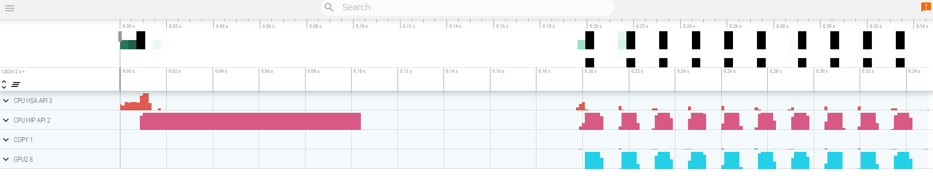Open a browser and go to [https://ui.perfetto.dev/](https://ui.perfetto.dev/). Click on `Open trace file` in the top left corner. Navigate to the `results.json` you just downloaded. Use the keys WASD to zoom in and move right and left in the GUI ``` Navigation w/s Zoom in/out a/d Pan left/right ``` ![image](https://user-images.githubusercontent.com/109979778/225451481-46ffd521-2453-4caa-8d28-fa4e0f4c4889.png) Read about hardware counters available for the GPU on this system (look for gfx90a section) ``` less $ROCM_PATH/lib/rocprofiler/gfx_metrics.xml ``` Create a `rocprof_counters.txt` file with the counters you would like to collect ``` vi rocprof_counters.txt ``` Content for `rocprof_counters.txt`: ``` pmc : Wavefronts VALUInsts pmc : SALUInsts SFetchInsts GDSInsts pmc : MemUnitBusy ALUStalledByLDS ``` Execute with the counters we just added: ``` srun rocprof --timestamp on -i rocprof_counters.txt nbody-orig 65536 ``` You'll notice that `rocprof` runs 3 passes, one for each set of counters we have in that file. Contents of `rocprof_counters.csv` ``` cat rocprof_counters.csv ``` ## Omnitrace * Load Omnitrace Omnitrace is known to work better with ROCm versions more recent than 5.2.3. So we use a ROCm 5.4.3 installation for this. ``` module load craype-accel-amd-gfx90a module load PrgEnv-amd module use /pfs/lustrep2/projappl/project_462000125/samantao-public/mymodules module load rocm/5.4.3 omnitrace/1.10.3-rocm-5.4.x ``` * Allocate resources with `salloc` `salloc -N 1 --ntasks=1 --partition=small-g --gpus=1 -A project_465000644 --time=00:15:00` * Check the various options and their values and also a second command for description `srun -n 1 --gpus 1 omnitrace-avail --categories omnitrace` `srun -n 1 --gpus 1 omnitrace-avail --categories omnitrace --brief --description` * Create an Omnitrace configuration file with description per option `srun -n 1 omnitrace-avail -G omnitrace.cfg --all` * Declare to use this configuration file: `export OMNITRACE_CONFIG_FILE=/path/omnitrace.cfg` * Get the training examples: `cp -r /project/project_465000644/Exercises/AMD/HPCTrainingExamples/ .` * Compile and execute saxpy * `cd HPCTrainingExamples/HIP/saxpy` * `hipcc --offload-arch=gfx90a -O3 -o saxpy saxpy.hip` * `time srun -n 1 ./saxpy` * Check the duration * Compile and execute Jacobi * `cd HIP/jacobi`  * Now build the code * `make` * `time srun -n 1 --gpus 1 Jacobi_hip -g 1 1` * Check the duration #### Dynamic instrumentation * Execute dynamic instrumentation: `time srun -n 1 --gpus 1 omnitrace-instrument -- ./saxpy` and check the duration  * About Jacobi example, as the dynamic instrumentation wuld take long time, check what the binary calls and gets instrumented: `nm --demangle Jacobi_hip | egrep -i ' (t|u) '` * Available functions to instrument: `srun -n 1 --gpus 1 omnitrace-instrument -v 1 --simulate --print-available functions -- ./Jacobi_hip -g 1 1` * the simulate option means that it will not execute the binary #### Binary rewriting (to be used with MPI codes and decreases overhead) * Binary rewriting: `srun -n 1 --gpus 1 omnitrace-instrument -v -1 --print-available functions -o jacobi.inst -- ./Jacobi_hip` * We created a new instrumented binary called jacobi.inst * Executing the new instrumented binary: `time srun -n 1 --gpus 1 omnitrace-run -- ./jacobi.inst -g 1 1` and check the duration * See the list of the instrumented GPU calls: `cat omnitrace-jacobi.inst-output/TIMESTAMP/roctracer.txt` #### Visualization * Copy the `perfetto-trace.proto` to your laptop, open the web page https://ui.perfetto.dev/ click to open the trace and select the file #### Hardware counters * See a list of all the counters: `srun -n 1 --gpus 1 omnitrace-avail --all` * Declare in your configuration file: `OMNITRACE_ROCM_EVENTS = GPUBusy,Wavefronts,VALUBusy,L2CacheHit,MemUnitBusy` * Execute: `srun -n 1 --gpus 1 omnitrace-run -- ./jacobi.inst -g 1 1` and copy the perfetto file and visualize #### Sampling Activate in your configuration file `OMNITRACE_USE_SAMPLING = true` and `OMNITRACE_SAMPLING_FREQ = 100`, execute and visualize #### Kernel timings * Open the file `omnitrace-binary-output/timestamp/wall_clock.txt` (replace binary and timestamp with your information) * In order to see the kernels gathered in your configuration file, make sure that `OMNITRACE_USE_TIMEMORY = true` and `OMNITRACE_FLAT_PROFILE = true`, execute the code and open again the file `omnitrace-binary-output/timestamp/wall_clock.txt` #### Call-stack Edit your omnitrace.cfg: ``` OMNITRACE_USE_SAMPLING = true; OMNITRACE_SAMPLING_FREQ = 100 ``` Execute again the instrumented binary and now you can see the call-stack when you visualize with perfetto. ## Omniperf * Load Omniperf: Omniperf is using a virtual environemtn to keep its python dependencies. ``` module load cray-python module load craype-accel-amd-gfx90a module load PrgEnv-amd module use /pfs/lustrep2/projappl/project_462000125/samantao-public/mymodules module load rocm/5.4.3 omniperf/1.0.10-rocm-5.4.x source /pfs/lustrep2/projappl/project_462000125/samantao-public/omnitools/venv/bin/activate ``` * Reserve a GPU, compile the exercise and execute Omniperf, observe how many times the code is executed ``` salloc -N 1 --ntasks=1 --partition=small-g --gpus=1 -A project_465000644 --time=00:30:00 cp -r /project/project_465000644/Exercises/AMD/HPCTrainingExamples/ . cd HPCTrainingExamples/HIP/dgemm/ mkdir build cd build cmake .. make cd bin srun -n 1 omniperf profile -n dgemm -- ./dgemm -m 8192 -n 8192 -k 8192 -i 1 -r 10 -d 0 -o dgemm.csv ``` * Run `srun -n 1 --gpus 1 omniperf profile -h` to see all the options * Now is created a workload in the directory workloads with the name dgemm (the argument of the -n). So, we can analyze it ``` srun -n 1 --gpus 1 omniperf analyze -p workloads/dgemm/mi200/ &> dgemm_analyze.txt ``` * If you want to only roofline analysis, then execute: `srun -n 1 omniperf profile -n dgemm --roof-only -- ./dgemm -m 8192 -n 8192 -k 8192 -i 1 -r 10 -d 0 -o dgemm.csv` There is no need for srun to analyze but we want to avoid everybody to use the login node. Explore the file `dgemm_analyze.txt` * We can select specific IP Blocks, like: ``` srun -n 1 --gpus 1 omniperf analyze -p workloads/dgemm/mi200/ -b 7.1.2 ``` But you need to know the code of the IP Block * If you have installed Omniperf on your laptop (no ROCm required for analysis) then you can download the data and execute: ``` omniperf analyze -p workloads/dgemm/mi200/ --gui ``` * Open the web page: http://IP:8050/ The IP will be displayed in the output ## MNIST example This example is supported by the files in `/project/project_465000644/Exercises/AMD/Pytorch`. These script experiment with different tools with a more realistic application. They cover PyTorch, how to install it, run it and then profile and debug a MNIST based training. We selected the one in https://github.com/kubeflow/examples/blob/master/pytorch_mnist/training/ddp/mnist/mnist_DDP.py but the concept would be similar for any PyTorch-based distributed training. This is mostly based on a two node allocation. * Installing PyTorch directly on the filesystem using the system python installation. `./01-install-direct.sh` * Installing PyTorch in a virtual environment based on the system python installation. `./02-install-venv.sh` * Installing PyTorch in a condo environment based on the condo package python version. `./03-install-conda.sh` * Installing PyTorch from source on top of a base condo environment. It builds with debug symbols which can be useful to facilitate debugging. `./04-install-source.sh` * Testing a container prepared for LUMI that comprises PyTorch. `./05-test-container.sh` * Test the right affinity settings. `./06-afinity-testing.sh` * Complete example with MNIST training with all the trimmings to run it properly on LUMI. `./07-mnist-example.sh` * Examples using rocprof, Omnitrace and Omniperf. `./08-mnist-rocprof.sh` `./09-mnist-omnitrace.sh` `./10-mnist-omnitrace-python.sh` `./11-mnist-omniperf.sh` * Example that debugs an hang in the application leveraging rocgdb. `./12-mnist-debug.sh`

Read more

Omniperf Advanced - part 2 - Performance Analysis Tools for AMD GPUs, CRAY User Group Tutorial 2024

Omniperf - Performance Analysis Tools for AMD GPUs, CRAY User Group Tutorial 2024

Omnitrace - Performance Analysis Tools for AMD GPUs, CRAY User Group Tutorial 2024

AI and ML exercises