# Driver2vec: Driver Identification from Automotive Data

:::info
**Group 75**
David Gomes (5624940) - [e-mail]
Parinith Iyer (5219027) - [e-mail]
Ricardo Valadas (5386632) - [e-mail]
:::
## Introduction
It might not be difficult to remember a situation where we had to drive a vehicle that was not our own. And even though it happens frequently, it is rarely a joyful feeling (unless it is a Ferrari). Beyond the burdening task of adjusting the car seat and mirrors, the driving experience is worsened simply because we are not used to the pedal or steering wheel sensitivity. Given this, identifying the operator of a vehicle is a task that enables a large range of potential uses. Starting from a customized adaptation of vehicle settings, it could also be used to alert the owner of possible theft.

The use of biometric devices could be a solution to this problem. However, the increasing concern with privacy protection suggests that other alternatives should be considered. One of them is taking advantage of the several sensors that modern cars are nowadays equipped with.

In this blog post we present a reproduction of the "Driver2vec: Driver Identification from Automotive Data" paper by Yang et al. (2021) [1]. In their approach, the authors transform a short time series of the sensors' data to an embedding that is representative of the driver. This embedding is then fed to a classifier to identify the user.

Even though part of the code was available online, we decided to attempt a full replication from scratch. There were two main reasons for this. Firstly, the code was poorly documented, which made it difficult to understand how the deep learning architecture was implemented. Secondly, only a small percentage of the data was made available. As we will explain later, this motivated a departure from the original paper approach, which meant the code would eventually have to be adjusted in order to accomodate this.

Our approach has the final objective of reproducing the feature ablation study presented in table 5. This is done by comparing the pairwise (2-way) accuracy after removing different groups of sensors.

*Table 5 from [1], showing the feature ablation study*.

## Methods
The *Driver2vec* architecture can be divided in two sequential parts:
1. The first block, which is the core of the model, corresponds to a time-series processing. For simplicity, we will refer to this block from now on as the **embedding model**. It receives a 10-second excerpt of 31 sensor features, sampled at 100Hz, which is processed in two parallel stages:

- The input is fed into a Temporal Convolutional Network (TCN) to generate an embedding vector of size 32.
- The same input is also transformed using the Haar wavelet, in order to capture information from the frequency domain. This transformation results in a vector of length 30.

2. The second block corresponds to a classification task to perform the driver identification. It uses LightGBM, which is an open source implementation of gradient boosting decision trees. We will refer to this block simply as **LightGBM**. The two vectors resultant from the embedding model are concatenated into a single 62-dimensional embedding, which is then fed into the LightGBM to predict the correct driver.

*Deep learning architecture of Driver2vec. This diagram is based on figure 1 from [1]*.

The following subsections specify how this architecture was reproduced and trained. We also enumerate the assumptions made where the paper lacked detailed information.

### 1. Data Processing
The authors of the paper state that their dataset included 15 minutes of test drives on a simulator for 51 different users, across 4 road scenarios ("highway", "suburban", "tutorial", "urban"). This summed to more than 15 hours of driving. However, only a very small portion of this data was made publicly available.

The sample dataset only contained data for 5 users in the 4 scenarios. Additionally, 19 of the 20 *(user, scenario)* combinations had 10 seconds of driving, and one of them *(user 3, "tutorial" scenario)* had just over 3 seconds. This meant that we only had 19 *10-second* inputs to train and test the model, which was remarkably little to obtain any valid results.

The solution we encountered to this problem was to use *2-second* snippets instead. The paper experimented this solution and warned for a reduction in model performance. This is an intuitive conclusion, since it is expected that a shorter time-series contains less information to distiguish drivers. In spite of that, we decided it was beneficial to trade a less informative input for more data.

An obvious implementation of this solution would be to divide the *10-second* data into 5 *2-second* sequences. This would result in 96 input samples (not 100 samples because *(user 3, "tutorial" scenario)* only yields 1 sample instead of 5). However, we decided to follow a strategy that is presented in Appendix 4 of the paper.

This strategy overlaps some instants of consecutive samples to increase the amount of data. Each sample is drawn with an interval gap of 0.4 seconds. Therefore, from a *10-second* snippet, we can obtain 21 samples instead of only 5. A scheme of this strategy is shown below.

*Scheme of the strategy used to sample 2-second intervals from a 10-second input. It was used a 0.4 seconds interval gap*.

In total, we were able to extend the initial 19 *10-second* inputs to 403 *2-second* samples. This data was divided in a 8:2 ratio for training and testing. We made sure that both the training and testing datasets had the inputs evenly represented by the different users and scenarios.

### 2. Temporal Convolutional Network (TCN)

Reading the original paper [1], there was not a lot of details about the workings of the TCN or the steps to build one. We mainly researched a lot on the internet to learn the properties and the structure of the TCN. In particular [an article by Francesco Lassig](https://unit8.com/resources/temporal-convolutional-networks-and-forecasting/) [2] presented a very clear and detailed explanation of the working and construction of a TCN. We based our TCN on the same model presented.

*Architecture of the TCN from Francesco Lassig's article [2]*

We also calculated the number of residual blocks to use with the formula [2]:

$$layers=\Biggl\lceil\log_2\bigg(\frac{(input\_length-1)\cdot(dilation\_base-1)}{(kernel\_size-1)\cdot2} - 1\bigg)\Biggr\rceil$$

Following the paper, we chose a dilation base of 2, and a kernel size of 16. The only deviation, due to the smaller data samples, was the input length of 200 (2 seconds of driving sampled at 100Hz) instead of 1000. In order to develop the basic causal conventional layers, the Conv1d function from the torch.nn module plus left zero-padding were used. This way it was possible for the last element of the sequence in the last convolutional layer of each basic layer block to have a receptive field of all the previous timesteps.

Finally, the output embedding of the TCN was a 32-size vector, however, the input samples only had 31 features. Therefore, it needs to be chosen a layer where the change in feature space occurs. Neither the paper nor the code explicitely refer to this, so the group decided to make this change in the first basic layer of the first residual block (refer to the figure above). Since there are residual connections in each residual block, this causes the input to have a different size from the output in this particular case. In order to fix this, a convolutional block of 1x1 was used to map the 31 feauture input to a 32 feature vector. From this layer, all consecutive ones already use the 32-dimensional feature space not being necessary to perform the additional 1x1 convolution.

### 3. Haar Wavelet Transformation

Similar to the TCN, the details about the implementation of this stage were not covered in the paper. Through our research, we found that a level-1 discrete wavelet transform (DWT) needs to be used for our implementation. This transform converts an input tensor to two tensors halved in size. These resultant tensors capture the frequency and location information. The output tensors are referred to as the approximation and detail coefficients [3].

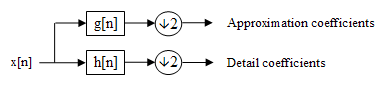
*Level 1 Discreet wavelet transform [3]*

The specific of the $g[n]$ and the $h[n]$ filters depend on the type of the DWT. In our caase, we use the Haar wavelet transform. In order to implement this, we used the [*pytorch_wavelets*](https://github.com/fbcotter/pytorch_wavelets) library by [*Fergal Cotter*](https://github.com/fbcotter) that is an implementation of various DWTs compatible for use in a pytorch network. After obtaining these 2 equal sized tensors from the DWT, each is parallely passed through a fully connected layer. It is important to note that the DWT does not have any trainable parameters as it is a predefined deterministic function. Finally, the input sample is converted to a 30-size vector output at this stage (15-size vector for each of the resultant tensor).

### 4. Embedding model training

The embedding model, which includes the TCN and the Haar wavelet transformation, was trained using triplet loss. In each step of the training, three samples $(x_a, x_p, x_n)$ are picked, where $x_a$ is an anchor, $x_p$ is a positive sample belonging to the same driver as $x_a$, and $x_n$ is a negative sample from a different driver.

The triplet loss function is defined as:

$$loss = max(0, D_{ap}^2 - D_{an}^2 + \alpha)$$

where $\alpha$ is a margin (hyperparameter) and $D_{ij}$ represents the $l_2$ distance between the resultant 62-dimensional embeddings from generic samples $x_i$ and $x_j$. The objective of triplet loss is to stimulate the network to place embeddings from the same driver close to each other and embeddings from different drivers far apart. In other words, it tries to achieve $D_{an}^2 \gg D_{ap}^2 + \alpha$.

The training procedure followed the same specifications as used in the paper. In particular, we used the Adam optimizer with a learning rate of $4\times 10^{-4}$ and a weight decay of $0.975$. The triplet loss margin $(\alpha)$ was set to $1$.

### 5. Gradient Boosting Decision Trees (LightGBM)
The LightGBM is used to classify the driver based on the 62-dimensional vector from the embedding model. Since this is an open source implementation, most of the overall structure of the classifier is already defined. The hyper-parameters were set as presented in Table 8 of [1], except for the metric, which we changed to "binary_logloss" since we were interested in pairwise evaluation. The remaining parameters that are not specified in table 8 were left with their default values.

*Hyper-parameters for LightGBM (table 8 from [1]). The metric was altered to "binary_logloss".*

After the embedding model was trained, we fed the same training dataset to the embedding model to predict the embeddings. These were then used as the input for the LightGBM training. Alongside the inputs, the corresponding driver labels were also fed to the classifier.

## Results

Once the whole model was trained, we evaluated performance in a pairwise setting. What this means is that instead of using directly the entire testing data, we predict separately in subsets from 2 drivers. We evaluate the accuracy of the model for each of the possible 2-way combinations among the 5 drivers. The mean accuracy is computed at the end.

In order to do the feature ablation study, we repeated this performance analysis several times. In each of them, a specific group of features was removed from the data. The objective of this study is to compare the relative importance of the features in the prediction accuracy.

Although the data we had at our disposal was quite insignificant compared to the authors, we saw significant similarities to the paper's results. In our experiments, we see that almost all settings which has some sensor groups removed perform worse than the group with all the sensor groups included.

| Removed sensor group | Pairwise accuracy (%) |
| ------------------------- | --------------------- |
| Speed, acceleraation only | 71.0 |
| Acceleration | 64.2 |
| Distance information | 66.7 |
| Gearbox | 72.4 |
| Lane information | 68.0 |
| Pedals | 69.3 |
| Road angle | 68.6 |
| Speed | 69.2 |
| Turn indicators | 68.8 |
| All features | 71.3 |

The `Gearbox` group is an outlier which acheived a performance increase of 1.1% compared to the inclusion of all features. In addition, the biggest drop we see in the accuracy is when we remove the acceleration information, showing that it is the most important group of features.

While we did not expect to see the results to be as good as the paper, we were successful in obtaining the similar trends. Acheiving an accuracy of 71.3% with the inclusion of all features, using only 0.35% of the original dataset, is certainly a promising outcome.

## Conclusion

The usage of the TCN and the discrete haar wavelets transform to process temporal data has proven to be a great approach. In addition, the use of triplet loss makes perfect sense and contributes towards acheiving proper seperation between different classes of multidimensional inputs.

Although the lack of training data was significant, the results acheived are better than expected, which highlights the strengths of the network architecture and might even make a case for using the original implementation in cases where data availability is less. The main plus-point in our opinion is that this implementation truly demonstrates the possibility of and paves the way for identification of drivers in a privacy-preserving manner, keeping personal data anonymous.

This reproducibility project was challenging, yet an insightful and postive experience. The techniques and results we obtained were inspiring and will definitely aid our technical decision in future projects.

----------------------------------------------
## References
[1] Yang, J., Zhao, R., Zhu, M., Hallac, D., Sodnik, J., & Leskovec, J. (2021). Driver2vec: Driver Identification from Automotive Data. https://arxiv.org/abs/2102.05234
[2] Francesco Lassig. Temporal Convolutional Networks and Forecasting. (2021) https://unit8.com/resources/temporal-convolutional-networks-and-forecasting/
[3] Wikipedia. Discrete wavelet transform. https://en.wikipedia.org/wiki/Discrete_wavelet_transform