Roadmap to Machine Learning 🦝

Welcome to the Machine Learning Roadmap by Programming Club IITK, where we will be giving you a holistic and hands-on introduction to the world of Machine Learning. The roadmap is divided into 8 weeks of content and each week progressively builds upon a new concept. The roadmap includes a lot of material and assignments, which while not trivial are definitely doable given the right amount of motivation and determination.

Also do remember, in case you face any issues, the coordies and secies @Pclub are happy to help. But a thorough research amongst the resources provided before asking your queries is expected :)

Before beginning, understand that the week allocation and order of topics covered is just a recommended order (Highly Recommended tho). For the first few weeks, we'd strongly recommend you to follow the order, since mathematics and basic foundations are quintessential for understanding working on any kind of model. Post that you can prolly play around with the order, take a few detours and come back. To explain how to do this in an a coherent fashion, we'll now give a run-through of the map.

Week 1 is basic python and libraries and week 2 covers basic mathematics, and the core fundamentals. Week 3 covers techniques important for improving ML pipelines. Follow these 3 weeks in order. 4th Week covers some of the most important algorithms, but they are not a prerequisite for week 4 (Intro to Neural Networks), so if you are too impatient to jump on the Neural Network and Deep Learning wagon, you can move to week 5 without completing week 4 (We'd recommend going the principled way tho). Moreover, week 7 (Unsupervised Learning) is pretty independent of all the weeks (except the first 3 weeks), so if you wish to explore Unsupervised Learning early, you can do that anytime. Week 6 covers some important topics like Optimization Algorithms, Feature Selection and Boosting Algorithms. You can go ahead with the first 2 subtopics without week 5, but Boosting Algorithms will require a strong understanding of Decision Trees so for that you'd have to go back to week 4. You can also cover Boosting Algorithms just after Ensemble Methods (Week 4, Day 4) if you're having fun learning about Decision Trees and wish to go deeper (ik, this was a pathetic attempt at cracking tree pun; just bear with for this not-so-short journey).

Coming to Python Libraries, PyTorch and Tensorflow are the most famous for Deep Learning, and ScikitLearn for ML in general. You'd learn sklearn as and when you progress the weeks, but after completing week 5 and the first 5 days of week 6, you'd have to pick one framework from PyTorch or Tensorflow. You can chose any one of them and getting a hang of one will also make it easier to understand the other. Once you're done with one framework, you can start building projects, learning the other framework, or exploring other specialized domains like CV or NLP.

One last tip before starting with your ML journey: It's very easy to scam one's way through their ML journey by having a false sense of ML mastery- by just copying code from Kaggle, GitHub or picking up models from modules directly. You can train an ML model in a single line using a scikitlearn function, but that does not quantify as "knowing" Machine Learning, but "using" a Machine Learning Model. One can only claim that they know Machine Learning if they understand the mathematics and logic behind the algorithm and process. Using modules and pre-trained models is efficient but doing that without knowledge is harmful. In a world where AI models like ChatGPT can help you code almost any ML problem effectively, having surface level awareness about existence of pre trained models and functions of various modules is just a waste of time and resources. At the same time, just theoretical knowledge does not help in solving real world problems. Stay balanced, optimize for understanding over a false sense of awareness and keep coding!

lmao, here are some memes (which you'd prolly understand by the end of this journey) to lighten up the mood 👾

🦝 Week 1 (Reviewing Python, introduction to numpy, pandas and matplotlib)

👾 Day 1: Get to know a bit about Machine Learning (A literature survey)

One must have a broad understanding of what the subject is at hand. Machine learning is a wide field with various domains. It would be really helpful if one goes through a couple of YouTube videos and/or blogs to get a brief hang of it, and its importance.
This video by TedEd is a must watch.
This blog is also an interesting read. It also cover the different types of machine learning algorithms you will face.
Another fun way to utilize ML:- the science behind lofi music

👾 Day 2 & Day 3: Learn a programming language, duh!

There are many programming languages out there, of which only two are suitable for ML, namely Python and R. We recommend any beginner start with Python. Why?

For one, it provides a vast selection of libraries, namely NumPy, pandas, sklearn, TensorFlow, PyTorch, etc., which are super helpful and require little effort for Machine Learning and data science.

Before starting, it is important to setup python in your device, using this as a reference.

Learning python is not hard. Here are a few resources which will teach you about the language swiftly:-

In case you come across a weird syntax or want to find a solution to problem, the official documentation is the best way to resolve the issues!

👾 Day 4: Start to get a hang of some of the inbuilt libraries like NumPy

Mathematics is the heart of Machine Learning. You will get a taste of this statement from Week 2. Implementing various ML models, loss functions, and confusion matrix need math. Mathematics is thus the foundation of machine learning. Most of the mathematical tasks can be performed using NumPy.

The best way to learn about libraries is via their official
documentation.

Other resources are as follows:-

Day 5: Proceed by exploring the other library, Pandas

Data is what drives machine learning. Analyzing, visualizing, and leaning information is an essential step in the process. For this purpose, Panadas comes to the rescue!

Pandas is an open-source python package built on top of Numpy and developed by Wes McKinney.

Like NumPy, Pandas has official documentation, which you may refer to here.
Other resources are as follows:-

👾 Day 6: Matplotlib - a powerful tool for visualization:

The average annual temperature above the industrial era around the globe

Both of the above figures show the same data. However, it is easier to visualize and observe patterns in the second image. (A scatter plot)

Matlotlib is a powerful library that provides tools (histograms, scatter plots, pie charts, and much more) to make sense of data.

The best source to refer to is the
documentation
in case of discrepancies.

Below are the links to some valuable resources covering the basics of
Matplotlib:-

👾 Day 7: Play around in Kaggle

Use this day as a practice field, to utilize all your skills you learnt. Head over to Kaggle and download any dataset you like. Apply the skills you procured and analyze trends in different data sets.
Here is a brief walkthrough of the UI.
All about Kaggle

🦝 Week 2 (Basic Mathematics for ML, KNN, Linear Regression)

Note, that I shall be constantly referring to Andrew NG's CS229 Course Lecture Videos, for they are the gold standard in any introductory Machine Learning course. The Lecture Notes of these course are pretty well made and can be referred to when needed. For additional notes, assignments, problem sets etc, refer the course site. Note that I shall not be always redirecting you to these videos since they are pretty mathematically rigorous. I shall be sometimes providing them as the main learning content, while other times adding them as Bonus Content, ie not having knowledge about those topics is completley fine but added knowledge and mathematical rigour will always help. In order to effetively absorb the videos, I recommend that you constantly refer to the aforeprovided lecture notes.

👾 Day 1: Descriptive Statistics

One must be comfortable with processing data using Python libraries. Before going further, let us recall some basic concepts of Maths and Statistics. Follow these resources:

Mean, Variance, Standard Deviation – Read theory from the book, Statistics, 11th Edition by Robert S. Witte, sections 4.1 - 4.6.
Gaussian Distribution – Read this blog.
Correlation in Variables – Read theory from the book, Statistics, 11th Edition by Robert S. Witte, Chapter 6.

👾 Day 2: Probability and Inferential Statistics

Knowledge of probability is always useful in ML algorithms. It might sound a bit of an overkill, but for the next two days, we will revise some concepts in probability. You can use your JEE Notes or cover theory from the book, Statistics, 11th Edition by Robert S. Witte, sections 8.7 - 8.10. Go through important theorems like Bayes' Theorem and Conditional Probability. Audit the Coursera Inferential Statistics Course for free and complete Week 1 up to CLT and Sampling.

👾 Day 3: Inferential Statistics Continued

Complete the remaining portion of Week 1 and Week 2 of the Inferential Statistics course. You can also use the book, Statistics, 11th Edition by Robert S. Witte, as a reference.

👾 Day 4: Intro to ML and Classification using KNNs

The common problems you would attempt to solve using supervised machine learning can be categorized into either a regression or a classification one. For example, predicting the price of a house is a regression problem, while classifying an image as a dog or cat is a classification problem. When you are outputting a value (real number), it is a regression problem, while predicting a category (class) is a classification problem. For a better understanding, you can refer this blogs on classification vs regression.

Apart from this classification, Machine Learning Algorithms can be broadly categorized into Supervised, Unsupervised, Semi-Supervised and Reinforcement Machine Learning. In supervised machine learning, labeled datasets are used to train algorithms to classify data or predict outcomes accurately. This means that the data provided to you have some kind of label or information attached, and this label is the value which the Algorithm has to learn to predict. For instance, feeding a dataset with images of cats and dogs, with each image labelled as either a cat or a dog into an algorithm which learns how to classify an image into a cat or a dog will come under Supervised Machine Learning.
Unsupervised machine learning, uses machine learning algorithms to analyze and cluster unlabeled datasets. These algorithms discover hidden patterns or data groupings without the need for human intervention. For instance, an algorithm which takes unlaballed images of cats and dogs as inputs, analzyes the similarities and differences between different types of images and forms clusters (or groups), wherein dogs belong to a given cluster and cats belong to another cluster is an example of unsupervised learning. This usually involves transforming the information, mapping the transformed information into some n-dimensional space and then using some similarity metrics to cluster the data. New data can be placed in the cluster by mapping it in the same space.

As the name suggests, Semi Supervised learning lies somewhere between supervised and unsupervised learning. It uses a smaller labeled data set to guide classification and feature extraction from a larger, unlabeled data set. Semi-supervised learning can solve the problem of not having enough labeled data for a supervised learning algorithm.

Reinforcement Learning algorithms form policies and learn via trial and error. Whether the policy is correct or wrong is determined via positive or negative reinforcements provided to the agent on completion of certain tasks (Similar to how you are appreciated when you get a great rank in JEE Advanced, but prolly scolded or beaten by your parents when you're caught consuming drugs). This process can be discrete or continuous. For instance, building an agent to play games like Flappy Bird or Pokemon.
For a better understanding of these classifications, refer to this article by GfG and this page by javapoint.

Now that we have a high level idea of how the domain of Machine Learning looks like, let's start understanding some algorithms.

KNNs are one of the first classification algorithms. Watch the first 5 videos of this playlist to know more. This would be a good point to implement the KNN Algorithm on your own, only using NumPy, Pandas and MatPlotLib. This will not only help you in understanding how the algorithm works but also help in building programming logic in general.

Building algorithms from scratch is important, but using modules to implement algos is fast and convenient when an alteration in the algo is not required. Try to implement a KNN via SciKitLearn by following this tutorial.

👾 Day 5 and 6: Linear Regression and Gradient Descent

A hypothesis function was the function that our model is supposed to learn by looking at the training data. Once the model is trained, we are going to feed unseen data into hypothesis function and it is magically going to predict a correct (or nearly correct) answer!

The hypothesis function is itself a function of the weights of the model. These are parameters associated with the input features that we can tweak to get the hypothesis closer to the ground truth.

But how do we ascertain whether our hypothesis function is good enough? That's the job of the cost function. It gives us a measure of how poor or how wrong the hypothesis function is performing in comparison to the ground truth.

Here are some commonly used cost functions:
https://www.javatpoint.com/cost-function-in-machine-learning

Now, we have a function we need to minimize and a function (cost function) that we need to predict (hypothesis function). The Cost function usually draws a comparison between the actual result and the predicted result. Since the predicted result is obtained by puttin the values of the features in the hypothesis function, the cost function contains in it the hypotesis function. Moreover, since we are minimizing the cost function, it is intuitive to make its derivative zero in order to get the values for which minimum error (ie, minimum cost function) is achieved. This is done via an algorithm called Gradient Descent.

Gradient descent is simply an algorithm that optimizes the weights of the hypothesis function to minimize the cost function (i.e., to get closer to the actual output). Gradient Descent is used to minimize the objective function by updating the parameters (which are usually all the weights and biases of the neural network) in a direction of maximum descent. That is, the parameters are updated in the direction of the negative gradient of the objective function. The gradient of the parameters multiplied by the learning rate (which is a hyperparameter set usually via heuristic approaches like grid search or Bayesian optimization) is subtracted from the parameters, and this process is iterated until a minimum is reached. The learning rate determines the size of the steps taken. A larger learning rate can lead to skipping the minima and aimless oscillations throughout the function and a small learning rate can lead to a huge number of steps and an extremely high amount of training time.

A major problem with Batch Gradient Descent is that it performs redundant computations because it calculates the gradients for similar training examples before updating the parameters, hence increasing the training time. The problem of redundancy is solved by Stochastic Gradient Descent.

As opposed to Vanilla Gradient Descent, Stochastic Gradient Descent updates the parameters after evaluating the gradients for each training example. Hence, it updates the parameters before evaluating the gradient for other similar training examples in the dataset, so the training speed increases.
But, since only one training sample is used for a single update, the fluctuations in cost function over the epochs are very high. There is a lot of noise in the graph of Cost Function vs number of epochs but the smoothened graph is usually a reducing graph.
It is easier for the SGD to reach a better minima due to a greater amount of fluctuations as opposed to VGD wherein the cost function reaches the nearest local minima. But these fluctuations can also lead to the function overshooting but this is usually solved by gradually reducing the learning rate towards the end of the training. Can we find a middle ground which captures the benefits of Stochastic as well as Vanialla Gradient Descent?

Mini Batch Gradient Descent tries to incorporate the best of both, Batch GD and SGD by dividing the training dataset into smaller batches and then updating the parameters after evaluation of gradients of the training samples in each mini-batch. The updated parameters are the difference between the previous parameters and the product of the learning rate and average gradients of the training samples in the mini-batch. This approach reduces the variance which is observed in SGD which leads to stable convergence and is computationally more efficient than Batch GD as it updates the parameters more frequently.

In future sections, we will dig deep into the problems which might arise during Gradient Descent and how the algorithm can be optimized. Now, since we have an idea about the fundamental concepts, let's delve into one of the simplest, yes widely used algorithm utilizing them: Linear Regression.

Go through this article on linear regression. For a deeper intuition, watch this video. You can refer to this, this and this for a better understanding of Gradient Descent.

This would be a good time to program Linear Regression from scratch by only using Numpy, Pandas and MatPlotLib. Before that, in order to structure your code effectively, it is imporant to understand Object Oriented Programming, which you can learn from here. Once you've gone through OOPs, you are ready to code your own linear regression model. Use this dataset for training and testing the model.

Follow this article to understand the implementation using various libraries. If you are further interested, you may see Statistics, 11th Edition by Robert S. Witte, Chapter 7.

For those who are curious to delve into the intricacies and maths behind LR and GS, you can watch this video by Andrew NG.

👾 Day 7: Preparation for Next Week

Towards the end of the week, let us revise some tools in linear algebra. This has some motivation regarding the content. Revise Vectors, Dot Product, Outer Product of Matrices, Eigenvectors from MTH102 course lectures here. Revise some concepts on multivariable mathematics (MTH101) here.

🦝 Week 3 (EDA, Cross Validation, Regularizations)

This week, we shall deviate a bit from Machine Learning Algorithms and learn about various techniques which help in making ML Pipelines more effective and improve the accuracy of the models. These include, but are not limited to Exploratory Data Analysis, preprocessing techniques, Cross Validation and Regularizations.

👾 Day 1: Exploratory Data Analysis (EDA)

Lets first understand the purpose of EDA in ML. The purpose of EDA as the name suggests is to understand the datasets, getting to know what useful comes out from it. Discovering patterns, spotting anomalies etc are also its part. It becomes very essential to do EDA For better understanding lets go through the articles below.

https://www.ibm.com/topics/exploratory-data-analysis
https://www.analyticsvidhya.com/blog/2021/08/exploratory-data-analysis-and-visualization-techniques-in-data-science/
This video goes well with the first link.
Finally see this to understand how to do EDA.
For Practice you can surely try doing EDA on datasets available on Kaggle.

👾 Day 2: Visualizing things with Seaborn

Seaborn is a robust Python library designed for data visualization, built on top of Matplotlib. It offers a high-level interface for creating visually appealing and informative statistical graphics, making it an ideal tool for exploratory data analysis (EDA). With Seaborn, you can generate complex visualizations with minimal code, allowing you to focus more on deriving insights from the data rather than on coding details. The library includes built-in themes and color palettes that enhance the visual quality of your plots effortlessly.

Seaborn simplifies the creation of common plot types such as histograms, bar charts, box plots, and scatter plots, while also providing advanced visualization options like pair plots, heatmaps, and violin plots. These advanced techniques are particularly useful for uncovering relationships and patterns within the data. Seamlessly integrating with Pandas data structures, Seaborn makes it easy to visualize data frames directly. Overall, Seaborn is an essential tool for data scientists and analysts, significantly improving their ability to understand and communicate data insights effectively.

The best source for learning about a python library is always its official Documentation. Here is its link.
Sometimes it may feel complicated and difficult to directly learn from the documentation. To ease the process. First go through the below links and for further learing, doubts or assistance refer to the documentation.

https://www.geeksforgeeks.org/introduction-to-seaborn-python/
You can see this or this whichever seems better to you. These are tutorials for Seaborn.
If looking for a youtube tutorial this may help.
When you are done and confident you can surely try applying your learnt skills on kaggle datasets.

👾 Day 3: Data Preprocessing

Data preprocessing involves transforming raw data into a format suitable for analysis and modeling. This step is crucial as it improves the quality of data and enhances the performance of machine learning models. More then just quality and performance, it is sometimes necessary to preprocess data so that we can feed it in machin elearning pipeline or else errors swarp around while running the code.
Important practices under Data Preprocessing include

Handling Missing Values: Missing data can introduce bias and reduce the accuracy of your machine learning models. Ignoring missing values can lead to misleading results because most algorithms are not designed to handle them. Properly addressing missing values ensures the integrity of your dataset and enhances the performance of your models. Follow this to understand how to do it.
Standardization and Normalization: Most machine learning algorithms require numerical input. Categorical data needs to be converted into a numerical format to be processed by these algorithms. Encoding categorical variables allows the model to interpret and learn from the data correctly.

👾 Day 4: Evaluation Metrics, Fairness and Bias

👾 Day 5: Data Splits and Cross Validation

Every Model has to be trained on some data and to evaluate how well it captures the generalized pattern, it is to be evaluate uning an unexplored data. The train data is used for training, and test data is used for testing the model.
But what will you do if the model performs well on the training data but pathetically on the test data. Such a situation is called Overfitting wherein the model captures the patterns of the training data points very well, but the general pattern is not rrecognized. To prevent this, we can use the "validation" data set. The splitting of data into the train, validation and test datasets is called the train validation test split.

This split helps assess how well a machine learning model will generalize to new, unseen data. It also prevents overfitting, where a model performs well on the training data but fails to generalize to new instances. By using a validation set, practitioners can iteratively adjust the model’s parameters to achieve better performance on unseen data. More on this later. On the basis of the need this split can be an 80-10-10, 70-15-15 or 60-20-20 split (usually a larger training set is preferred).

There are certain values (formally called, parameters) for instance the batch size or step size in the case of linear regression which need to be manually set by the user before the training of the model. Such parameters are called Hperparameters, and it is important to set them in such a manner that the model generalizes. The process of evaluating such values is called Hyperparameter tuning and is done via Cross Validation and iterative sampling. Cross Validation requuires using the Validation Dataset to continuously validate the model during and select the best values of Hyperparameters.

Watch this video to understand the theory behind hyper parameter tuning using cross validation, and this for implementing Cross Validation and Grid Search via SciKitLearn.

Iterative Sampling for Hyperparameter tuning can be done via various methods like Grid Search (Just bruteforcing your way through all the values. This is very expensive in terms of time and might miss out certain values in case of countinuous values since we'd need to have some step size), Randomized Search (Might be faster, but way more inefficient because as the name suggests,it's random) and Bayesian Optimization.

Bayesian Optimiziation uses Bayes Theorem, Surrogate Functions and Gaussian Regression in order to predict the next best parameter value. It is fairly easy to implement via SciKitLearn, but completely understanding the mathematics behind it might be pretty complex and can be skipped at this point. But for the stats and math entusiasts, you can refer this article for understanding the theory and this for implementing it from scratch.

👾 Day 6: Regularization

Yesterday we learnt about overfitting and why it is bad for any Machine Learning model. To solve this problem, let's ask the question as to why overfitting occurs? Because it gives too much importance to the training data points and tries to fit a curve which passes through all the points. So, we need to reduce the importance given to these exact points and account for some sort of variance as well. This can be done by by adding a penalty term to the loss function, discouraging the model from assigning too much importance to individual features or coefficients. This technique is called Regularization.

There primarily exist 3 types of regularizatins: Lasso (L1), Ridge (L2) and Elastic Net (L1-L2) regularizations. The only difference amongst them is what kind of penalty term is added.

This is a great article which would prodive you a pretext (Bias, Variance, Overfitting, Underfitting) as well as explain the penalty terms of different types of regularizations.

Now go back to the Linear Regression Model you built from scratch and try to incorporate these 3 regularizations (separately, obviously) in the model. Train them and compare the accuracies. Try to tune the regularization based hyperparameters using Bayesian Optimization and Cross Validation. What conclusion do you draw from the results and comparisons? Is the change in accuracy significant and in the positive direction? Why or why not?

👾 Day 7: Bonus and Revision

Week 4 will actively use the fundamentals covered in Week 2, so I'd recommend you to go through your notes and revise gradient descent and linear algebra. If you're confident with these topics, you can cover these bonus topics from the second lecture of Stanford CS229. I've explained these topcis in brevity for introduction, but I recommend you to go through the lecture for understanding.

🐼 Locally Weighted Regression

If a target(output)-feature relationship is non linear, in that case linear regression produces low accuracy score because it can only capture linear relationships. One workaround could be manually adding a feature that is related non linearly with the initial feature (for instance, \(x^n\)). As you'd remember, this is called feature engineering and helps a lot in capturing non linearities. But the issue is that this reuires a huge amount of EDA and the feature created might not be very accurate because this is a manual procedure. Hence, for these kinds of problems, we use locally weighted regression.

In Locally weighted regression, if we want to predict the target (output value) for a given set of features (input vector), we try to fit our weights to minimize a loss function which a weighted loss function. This weight is determined by the proximity of a point to the given input vector. Since we are giving more weight to proximate point and the weight is exponential in nature with respect to distance, the likelohood of accuracy is less. Such type of learning algorithm is called a Parametric learning algorithm because the time required to make the prediction is propotional to the size of the training data.

🐼 Probabilistic Interpretation

Have you other wondered why the Loss function we select is a Mean Square Loss? Why isn't this linear or cubic? You'd read at various places that this is to make it more computationally efficient, or to make the derivatives linear which makes things easy for us. This is correct but these are not the correct reasonings as to why Mean Square Loss is used, but these are just implications of using it. The correct reaoning is that when we use Maximum Likelihood Estimation. We chose the parameters (ie the weights) which maximize the Likelihood Function. Again, for mathematics and details, refer the video linked above.

🦝 Week 4 (Naive Bayes, Logistic Regression, Decision Trees)

By now you should have a grasp over what regression means. We have seen that we can use linear regression to predict a continuous variable like house pricing. But what if I want to predict a variable that takes on a yes or no value? For example, if I give the model an email, can it tell me whether it is spam or not? Such problems are called classification problems and they have very widespread applications from cancer detection to forensics.

This week we will be going over three introductory classification models: logistic regression, decision trees and Naive Bayes Classifiers. Note that devision trees can be used for both: regression and classification tasks.

👾 Day 1 - Logistic Regression

🐼 Logistic Regression Algorithm and Utility

The logistic regression model is built similarly to the linear regression model, except that now instead of predicting values in a continuous range, we need to output in binary, i.e., 0 and 1.

Let's take a step back and try to figure out what our hypothesis should be like. A reasonable claim to make is that our hypothesis is basically the probability that y=1 (Here y is the label, i.e., the variable we are trying to predict). If our hypothesis function outputs a value closer to 1, say 0.85, it means it is reasonably confident that y should be 1. On the other hand, if the hypothesis outputs 0.13, it means there is a very low probability that y is 1, which means it is probable that y is 0. Now, building upon the concepts from linear regression, how do we restrict (or in the immortal words of 3B1B - "squishify") the hypothesis function between 0 and 1? We feed the output from the hypothesis function of the linear regression problem into another function that has a domain of all real numbers but has a range of (0,1). An ideal function with this property is the logistic function which looks like this:

https://www.desmos.com/calculator/se75xbindy.
Hence the name logistic regression.

However, we aren't done yet. As you may remember we used the mean squared error as a cost function. However, if we were to use this cost function with our logistic hypothesis function, we run into a mathematical wall. This is because the resulting hypothesis as a function of its weights would become non-convex and gradient descent does not guarantee a solution for non-convex functions. Hence we will have to use a different cost function called binary cross-entropy.

Have a look at these articles:

We can now use gradient descent.

🐼 Implementation in Python

For a thorough understanding of how to use the above concepts to build up the logistic regression model refer to this article:
https://towardsdatascience.com/logistic-regression-detailed-overview-46c4da4303bc

One thing you must always keep in mind is that while learning about new concepts, there is no substitute for actually implementing what you have learnt. Come up with your own implementation for logistic regression. You may refer to other people's implementations.
This will surely not be an easy task but even if you fail, you will have learnt a lot of new things along the way and have gotten a glimpse into the inner workings of Machine Learning.

Some resources to help you get started:

Some datasets you might want to use to train your model on:

Iris Dataset - https://archive.ics.uci.edu/ml/datasets/iris
Titanic Dataset - https://www.kaggle.com/c/titanic/data
Bank Marketing Dataset - https://archive.ics.uci.edu/ml/datasets/bank+marketing#
Wine Quality Dataset - https://archive.ics.uci.edu/ml/datasets/wine+quality

🐼 Bonus

For mathematical representation, you can watch the relevant sections of the second lecture of Stanford CS229, and also explore NEWTONS METHOD for optimzation.

👾 Day 2: Gaussian Discriminant Analysis and Naive Bayes

Today's content is largely derived from Lecture 5 of CS229, so you're recommended to watch the lecture and refer to the notes. (Also, don't get fooled by the term "Naive", this algorithm is pretty smart; not as Naive as you 👾)

🐼 Generative v/s Discriminative Learning Algorithms

The algorithms we've explored so far (Linear Regression, Logistic Regression) model \(p(y|x;\theta)\) that is the conditional distribution of \(y\) given \(x\). These models try to learn mappings directly from the space of inputs \(X\) to the labels are called discriminative learning algorithms. The alfgorithms which model \(p(x|y)\) are called Generative Learning Algorithms. These Generative algorithms take a particular class label (\(y\)), and then learns how that class looks like (\(x\)) (essentially, \(p(x|y)\)). This when done iteratively helps the model to learn how the features of a given class look like.

🐼 Bayes Rule and it's applications

Let's use some High School probability to work on Generative Learning Algorithms.
\(p(x|y=1)\) models the distribution of features of class 1, and \(p(x|y=0)\) models the features of class 0. Now we can calculate \(p(x)\) using:\[ p(x) = p(x|y=1)p(y=1) + p(x|y=0)p(y=0) \] Now, we use the good ol' Bayes Rule: \[ p(y|x) = \frac{p(x|y)p(y)}{p(x)} \]

🐼 Gaussian Discriminant Analysis (GDA)

We assume that \(p(x|y)\) is distributed like the Multivariate Gaussian Distribution (A Multivariate form of the Bell Shaped Gaussian distribution). Refer to page

🐼 Naive Bayes Classifier

The Naive Bayes classifier applies Bayes' theorem with the "naive" assumption of independence between every pair of features.
In practice, we calculate the posterior probability for each class and choose the class with the highest probability as the predicted class.
It is naive as is does not preserve the sentence order, "Hardik drinks water" and "water drinks Hardik" are same to it.
Despite it being naive, it has been found to work well in tasks like spam detection and other binary classification tasks.

Types of Naive Bayes Classifiers

There are several types of Naive Bayes classifiers, each suited for different types of data:

Gaussian Naive Bayes: Assumes that the continuous features follow a Gaussian (normal) distribution.Gaussian Naive Bayes video
Multinomial Naive Bayes: Suitable for discrete data, such as word counts in text classification.Multinomial Naive Bayes video

You can also go through this Wikipedia article.

👾 Day 3: Decision Trees

Now let's move onto another interesting classification paradigm: the decision tree. Till now we have primarily looked into linear models, which are easily able to accurately model data which shows some form of linear pattern, or a pattern which is reducible to a linear problem. Today we shall be discussing a non-linear model.

This model is even more powerful and intuitive than logistic regression. You have probably used a decision tree unconsciously at some point in your life to take a decision. You'd have come across a meme which claims that Machine Learning is nothing but a huge collection of if statements and for loops and learning about Decision Trees will reinforce that claim. I'm not a huge fan of putting memes in roadmaps and documents (largely because they mess up the formatting and it just takes away the seriousness; which might be ironic coming from me for I have randomly used raccoon emoticons in the doc, but that's a story for another day 🦝), so I'm not including it here but you get the point.

For this topic, the main resource would be this playlist on classiciation and regression trees by the Muscial ML Teacher: Josh Starmer

In case you aren't familiar with what a tree is have a look at https://www.programiz.com/dsa/trees

Above is a decision tree someone might use to decide whether or not to buy a specific car

In an essence, you recursively ask questions (if-else statements) until you reach a point where you have an answer. In the dataset, we'll have a number of features, including continuous features and categorical features. How does the decision tree get to know what and how many questions to ask? More specifically the question(s) should be about which features(s)? Do we ask one question per feature or multiple questions? Do we ask any questions about a partiucalar feature at all? And in which order should questions be asked?

If you analyze these questions and how a human would answer these, you'd conclude that the answer to these questions is related to how much "information" do we gain about the output when we get the answer to a particular question. How do we quantify "information" mathematically such that we can use this "information metric" to somehow construct this tree. Statisticians have tried to encapsulate information objectively via certain metrics like Entropy, Gini Impurity, Information Gain etc. Go thorugh the following articles before proceeding.

Moving on to how to build a decision tree, refer to the following:

Concurrently, you can follow the following videos for intuitive understanding and visualization:

So far we have not really looked into much code. But as always no concept is complete without implementation.

You may refer to the following for help:

The following video presents a great pipeline to implement A Classficiation Tree Model:
https://www.youtube.com/watch?v=q90UDEgYqeI&list=PLblh5JKOoLUKAtDViTvRGFpphEc24M-QH&index=5

Finally, solve the Titanic challenge on Kaggle:
https://www.kaggle.com/competitions/titanic

Bonus: You can go through the first section of Lecture 10 of CS229 for a formal mathematical formulation of Decision Trees. This is not necessary coz after soo much practise and reading you'd have a decent understanding but if you have time to spare, this is definitely better than scrolling through dumb insta reels.

👾 Day 4: Ensemble Methods

Ensembling simply means combining the output of various models in a particular manner in an attempt to improve the accuracy of the combined (ensembled) model. Ensembling can include simple methods (like majority voting, weighted voting, simple averagin, weighted averaging), stacking, boosting, bagging etc. Refer to the following articles for understanding these ensemble learning methods:

We'll dive deep into Bagging today, and cover Boosting and various Boosting Algorithms later in Week 6. If you wish, you can cover it post Bagging as well. Follow these videos for Baggin:

Today was a light day, but be ready to go into the forest to encounter some Tygers 🐯

👾 Day 5: Random Forests

"Trees have one aspect that prevents them from being the ideal tool for predictive learning, namely inaccuracy"
~ The Elements of Statistical Learning

So what do we do? Combine tonnes of trees to create a forest! Simple enough? No!
We use Bagging (Bootstrapping and Aggregation) in order to combine multiple trees (those trees are not built like standard Decision Trees, but follow a specific procedure), an this forms a Random Forest. Go through the following videos to understand Random Forests:

Now try to implement Random Forests from scratch on your own!

Bonus: You can find the original research paper on Random Forests over here and an overview of the same in this Berkley Article. Following the research paper is tough and not really recommended at this level (Even I haven't read it), but for mathematical and theoretical insights, you can refer the overview.

👾 Day 6: Support Vector Machines

👾 Day 7: Kernel Methods

🦝 Week 5 (Perceptrons, Neural Networks, and an introduction to Tensorflow)

The next month of this roadmap will be devoted to Neural Networks and their applications.

👾 Day 1,2,3 - The perceptron and General Linear Models

(lmao there's a specific reason why 3 days have been allotted to a topic which is not widely talked about, so just try to stick with me for a few days; post that you'll feel like a different person 🙃🦝)
Content on of this week is largely derived from the fourth lecture of CS229, so you can constantly refer the video and the lecture notes for better understanding. Knowledge for Mathematical formulation of GLMs is recommended but not compulsory; it provides a great intuition behind similarity patterns in various ML algorithms and groups them under a larger class.

🐼 Perceptrons

The ultimate goal of Artificial Intelligence is to mimic the way the human brain works. The brain uses neurons and firing patterns between them to recognize complex relationships between objects. We aim to simulate just that. The algorithm for implementing such an "artificial brain" is called a neural network or an artificial neural network (ANN).

At its core, an ANN is a system of classifier units which work together in multiple layers to learn complex decision boundaries.

The basic building block of a neural net is the perceptron. These are the "neurons" of our neural network.

Do you see the similarity with logistic regression? What are the limitations of using the Perceptron Learning Algorithm? Do you think that Logistic regression is just a softer version of the Perceptron Learning Algorithm?

You'd notice that there is a fundamental similarity between the update functions of linear regression, logistric regression as well as the perceptron; with the only difference being in the hypothesis function part of the update. What does this signify? Is there a deeper correlation or is this just a coincidence? Let's explore further.

🐼 Exponential Families

For understanding exponential families, we'd have to understand basic probability distributions (which we covered in the second week) and the probabilistic interpretation of linear regression (refer the probabilstic interpretation of this video lecture for a refresher)

A refresher on probability distributions:Probability Distribution Function For Machine Learning
Bonus Material:Medium Article on Prob Distributioins for ML and DL

Note that Exponential Families and GLMs come under the probabilstic interpretation of Machine Learning (which you'd study in CS772: Probabilistic ML if you take the course (and get it lmao)) and is not at all important for building ML models of the level you'd be building as a beginner. But these become largely important when you delve deep into statistical modelling of data. So if you feel that this is boring or is taking a huge amount of time to understand, you can prolly move on to Day 2 and come back to this section later.

Anyways, back to the discussion. Recall that when we were trying to model data using linear regression, we approximated Y (the output) as a sum of a function of X and an error term \(\epsilon\). We assumed gaussian probability distribution about the mean 0 for the distribution of \(\epsilon\). Note that gaussian distribution is a specialized case of a class of functions called "exponential families", which are defined by:\[ p(y|\theta) = exp(\eta (\theta)T(y) + A(\theta)+B(y)) \] wherein:

\(y\) is the data
\(\theta\) are the parameters (which are to be altered, like weights and biases)
\(exp(B(y))\) is the base measure
\(\eta (\theta)\) is called the natural parameter
\(T(y)\) is the sufficient statistic
\(A(\theta)\) is the log-partition function or cumulant function.

You'd find different representations of the same thing at different places, but the form remains more or less same.

If you take specific values of the functions, and do some maniputlations to this function, you'd end up with famous distributions that we have studied, for instance, Gaussian (linear regression), Bernoulli (logistic regression), Poisson etc. Exponential families have several key properties that make them particularly important and useful in modeling data and machine learning:

Data Reduction: Exponential families have sufficient statistics \(T(x)\) that summarize all the information needed from the data to compute the likelihood. This means we can reduce the data to these statistics without losing information about the parameter estimation. Computation of likelihood is important, because as observed earlier, the maximum likelihood provides a method to evaluate the ideal cost function, which when extremized gives us the values of the parameters (weights and biases in case of NNs) which make the hypothesis approach the natural function.
Efficiency: Using sufficient statistics reduces the dimensionality of the problem, leading to more efficient computations.
Linear Combination: The natural parameters 𝜂(𝜃) and the sufficient statistics \(T(x)\) combine linearly in the exponent. This linearity simplifies the algebra involved in statistical inference.
Normalization: The log-partition function \(A(\theta)\) ensures that the probability distribution is properly normalized (i.e., integrates to 1). It also plays a crucial role in deriving other properties of the distribution.
Moments: The log-partition function helps in calculating the moments (mean, variance, etc.) of the distribution.
Simplified Algorithms: The mathematical properties of exponential families enable the development of efficient algorithms for parameter estimation (e.g., Maximum Likelihood Estimation, Expectation-Maximization).

CS229 lectures notes and lecture should be enough to understand exponential families. For a better understanding, refer to the following resources:

Sidenote: This Man Marius Hobbhahn is an absolute legend who primarily works on Bayesian ML and has written pretty insightful blogs on the mathematical aspect of ML. Moreover, he's a pretty successful debator. Do check out this website for intrinsically interesting stuff 🦝🙃

🐼 Generalized Linear Models

If you've made this section, first of all, Congratulations!, secondly it will be pretty simple for you to understand GLMs as they are just a way to model and apply exponential families. You'd have realized that Machine Learning is just abut finding a function/model which gives an approximately correct output when you input vector containig certain features; and modelling the same requires assuming some form of probability distribution because the world is largely how probabilties manifest (Quantum Mechanics ahem ahem 👾☠️👾). The way we DESIGN this model and make assumptions largely dictates the accuracy of this model. Let's talk more about this Design Philosophy, and Design Choises.

Consider a classification or regression problem where we would like to predict the value of some random variable y as a function of \(x\). To derive a GLM for this problem, we will make the following three assumptions about the conditional distribution of y given x and about our model:

\(y | x; θ\) ∼ ExponentialFamily(\(\eta\)). I.e., given \(x\) and \(\theta\), the distribution of
\(y\) follows some exponential family distribution, with parameter \(\eta\). This assumption manifests in linear regression as assuming that the error term \(\epsilon\) has a gaussian distribution about 0 with \(\sigma ^{2} = 1\).
Given \(x\), our goal is to predict the expected value of \(T(y)\) given \(x\). In most of our examples, we will have \(T(y) = y\), so this means we would like the prediction \(h(x)\) output by our learned hypothesis h to satisfy \(h(x) = E[y|x]\).
The natural parameter η and the inputs x are related linearly: \(\eta = \theta ^{T}x\). This is a crucial assumption, and can't really be justified per se at this level. So let's just assume that this is a "Design Choise" which just works out pretty well.

These three assumptions/design choices will allow us to derive a very elegant class of learning algorithms, namely GLMs, that have many desirable properties such as ease of learning. For understaning how Linear, Logistic and Softmax Regression can be modelled as GLMs, jump to page 30 of these notes. More on SoftMax in the next subsection

🐼 SoftMax Regression

👾 Day 4: Introduction to Neural Networks and Backpropagation

Moving on to how we build up a neural network from perceptrons.

https://medium.com/deep-learning-demystified/introduction-to-neural-networks-part-1-e13f132c6d7e

https://medium.com/ravenprotocol/everything-you-need-to-know-about-neural-networks-6fcc7a15cb4

You should also watch the first video in 3Blue1Brown's series on Neural Networks.

https://www.youtube.com/watch?v=aircAruvnKk&list=PLZHQObOWTQDNU6R1_67000Dx_ZCJB-3pi

Now you might be wondering how to train a neural network. We are still going to be using gradient descent (and its optimized forms) but to calculate the gradients of the weights we will be using a method called backpropagation.

https://machinelearningmastery.com/difference-between-backpropagation-and-stochastic-gradient-descent/

To get a visual understanding you are encouraged to watch the remaining 3 videos of 3B1B's series on Neural Networks.

https://www.youtube.com/playlist?list=PLZHQObOWTQDNU6R1_67000Dx_ZCJB-3pi

Refer to the following articles to get a feel of the mathematics under the hood.

https://towardsdatascience.com/deriving-the-backpropagation-equations-from-scratch-part-1-343b300c585a

https://towardsdatascience.com/understanding-backpropagation-algorithm-7bb3aa2f95fd

👾 Day 5: Debugging ML Models and Errors

Once again, like the first 3 days the content for this week is largely derived from CS229 lecture 13, and the same will be the base resource for the day.

Debugging ML model workflows is one of the most important skills, for a model more often than not, does not work for the first time (at least not accurately) you program it (unless, obv if you're just copy pasting a code from kaggle, GPT or blog, and in that case we won't really call it "building" a pipeline). Therefore,the stuff you learn today will be pretty useful in building real world applications and projects. So let's get started with some diagnostics and methods :)

🐼 Bias v/s Variance Diagnostic

In Week 3, we talked about two crucial metrics: Bias and Variance. In this section, we'll understad how they can be exploited for debugging ML models. For a quick refresher, you can go through this blog.

The learning curve (error v/s training set size) of a high variance model largely looks like this:

2 metrics to detect such a curve:

Test error decreases as training set size increases.
Large gap between training and test error

These metrics suggest, that to fix these issues, following tactics might be helpful:
a) Get more training examples, as test error decreases as training set size increases; so the test set graph might extrapolate
b) Try a smaller set of features. High variance in statistics means that the data points in a dataset are widely spread out from the mean, which is often due to a high set of features. So reducing the number of features might help.

Whereas the high bias counterpart looks as follows:

2 metrics to detect such a curve:

Training error is unacceptably high
There's a small gap between training and test error

Increasing the training set might not help as the error is largely constant of the training examples.

These metrics suggest, that to fix these issues, following tactics might be helpful:

Using a larger set of features, so that patterns are captures in a much better manner. After this, if the model has a high variance, increasing the number of training examples might help.
Try to quaitatively analyze the features, perform Exploratory Data Analysis, Data Preprocessing and Feature Engineering as these techniques might help in extracting features with better correlation.

🐼 The Optiization Problem v/s Maximization Problem Diagnostic

In any ML Problem, we try to maximize a particular function, and for maximizing that function, we use an optimization algorithm. In an application, the issue with our model design might either be a wrong choise of Cost Function, or a wrong choise of optimization algorithm. How do we identify what exactly is wrong?

Let's say we are trying to solve a problem and model A performs better than model B on a particular metric (metric which is important for your use case), but you need to deploy model B only, prolly because its exponentially faster or because model A has other inherent issues. How do we identify the problem. Let's say model B tries to optimize the cost function J. We don't really care about the cost function which A optmizies so let's keep that aside. \(\theta_A\) are the params of model A and \(\theta_B\) are params of B. There are 2 cases:
a) \(J(\theta_A) > J(\theta_B)\): This means that the optmization algorithm failed to converge, and we should prolly run the algorithm for more iterations or go for another optimization algorithm, like Newton's method.
a) \(J(\theta_A) <= J(\theta_B)\): This means that the optimization algorithm succeeded in optimizing the cost function, but the cost function selection is bad so we much change it. We can do this by either changing the cost function compeltely or altering the hyperparameters of the regularization (because that tweaks the cost function).

This is a theoretical overview of some of the commonly used diagnostics. For more detailed examples and workflows, go through the video linked in the beginning of the section.

👾 Day 6, 7: Implement a Neural Network from Scratch

Dedicate these two days to try to implement a neural network in python from scratch. Try to have one input, one hidden, and one output layer.

You may train your model on any of the datasets given in week 3.

https://towardsdatascience.com/an-introduction-to-neural-networks-with-implementation-from-scratch-using-python-da4b6a45c05b

🦝 Week 6 (Optimizations, Feature Selection, Boosting Algorithms)

👾 Day 1, 2: Optimization Algorithms

🐼 Problems with Vanilla Gradient Descent

There are multiple issues which arise when we implement Gradient Descent on complex (non quadratic) cost functions:

Local Minimas and Saddle Points: Loss Functions are convex in nature, which might lead to the Gradient Descent Algorithm converging at a nonoptimal local minimum. The networks usually get trapped at various saddle points and local minima. A greater issue is encountered with saddle points as they are surrounded by plateaus of similar error, making it extremely hard to escape from these points.
The difficulty is choosing an optimal learning rate: A low learning rate leads to extremely slow convergence and a high learning rate leads to difficulty in convergence as the function skips the minima and fluctuates and oscillates around the graph.
Non-Dynamic nature of training rate schedules: If we try to alter the training rate according to a pre-set schedule, we are not able to dynamically alter the training rate according to the dataset’s characteristics.
Application of same learning rate to all parameters: Certain weights and other parameters need not be updated to the same extent, but in vanilla gradient descent, all parameters are updated according to the same learning rate which might not be required.

In order to solve these problems, let's take a look at a few optimization techniques.

🐼 Momentum Based Optimization

Momentum-based optimization techniques make use of a term that contains information about the past values of the gradient in order to update the weights. The momentum-based gradient descent builds inertia in a direction in the search space to overcome the oscillations of noisy gradients. It uses Exponentially Decaying Moving Averages because the information about the older gradients is not as relevant as the information about the newer gradients.
\[ x_{k+1} = x_k − sz_k \] Where:
\[ z_k = \Delta f_k + βz_{k−1} \]

Here, \(z_k\) captures the information of the past gradients. The multiplication by \(\beta\) in this recursive function ensures that as the gradient gets older, its information is lost, that is its weight in the calculation in alteration of parameters reduces as a power of \(\beta\). This not only ensures that the number of steps in the optimization is reduced but also ensures that the model is not stuck in saddle points or local minima and it explores beyond these points also during descent.

This article gives a great insight into the inherent problems with Gradient Descent and provides the implementation of Momentum in Gradient Descent.

For Math nerds, this video by Legendary Mathematician Gilbert Strang (you might read/might have read his book on Linear Algebra for MTH113) provides a great mathematical understanding from a Linear Algebra perspective.

🐼 Nestrov Accelerated Gradient

A major issue with momentum-based optimization is that the model tends to overshoot because when it is about it reach the optimum value, it is coming down with a lot of momentum, which might lead to overshooting.
To solve this problem, Nestrov Accelerated Gradient tries to ”look ahead” to where the parameters will be to calculate the gradient. The standard momentum method first computes the momentum at a point and then takes a jump in the direction of the accumulated gradient, but as opposed to that Nestrov Momentum first takes the jump in the direction of the accumulated gradient and then measures the gradient at the point it reaches to make the correction. This additional optimization prevents overshooting. This is given by:\[ v_t = \lambda v_{t−1} + \eta \Delta J(\theta − \lambda v_{t−1}) \] where:\[ \theta = \theta − v_t \]

The following videos will provide and great visualization and intuitive understanding of NAG:
A 4 min quick visualization
Another great visualization

Try to code NAG from scratch.

🐼 Learning Rate Adaptation: Adagrad

The same learning rate might not be ideal for all parameters for an optimization algorithm, for sometimes it might need a higher rate to quickly descent, or sometimes it might require a lower rate. Adagrad is an optimzation algorithm that adapts the learning rate to the parameters, performing larger updates for infrequent and smaller updates for frequent parameters. Refer to this videos for a detailed explaination of how Adagrad works and then try to implement it from scratch.

🐼 Adam

Adam stands for Adaptive Moment Estimation. It is a method that computes adaptive learning rates for
each parameter. It aims to use the best of both worlds of using moments and using a learning rate custom to each parameter(based on their frequency). It maintains two moving average estimates of gradients and squares of gradients, and updates parameters using these estimates. It is preferred as the optimization algorithm for most Neural Networks because of the following reasons:

Adam converges faster compared to traditional optimization algorithms SGD due to its adaptive learning rate. By adjusting the learning rates individually for each parameter, Adam can make more
significant progress in optimizing the loss function.
Adam has found to work well across various deep learning architectures and tasks, including image classification, natural language processing, and reinforcement learning.
Adam has default hyperparameters that typically work well across different tasks and datasets, reducing the need for manual tuning.

For a detailed explanation of how Adam works, and its visualization refer to this video.

This Paper by Sebastian Ruder is a 🦝 MUST READ 🦝 and provides a great insight into Vanilla, Stochastic and Mini Batch Gradient Descent, their shortcoming and all momentum based optimized versions of Gradient Descent, ie NAG, Adagrad, Adadelta, RMSprop, Adam, AdaMax and Nadam. It then, goes on to provide comparative visualizations of these optimizations and proposes methods to parallelize and distribute the running of SGD. Lastly, it provides additional strategies for optimizing SGD like Shuffling and Curriculum Learning, Batch normalization, Early stopping and Gradient noise. If you wish to go deep into any of these subtopics, you can read the research papers cited in this paper and other references provided. I just stress enough on the importance of this paper and the amount of knowledge you'd gain by just understanding it.

For a summary and comparison of the important optimizers, refer to this and this

👾 Day 3: Feature Selection Techniques

Feature selection is a crucial process that helps in choosing the most important features from your dataset, reducing the feature space while preserving the essential information. This not only speeds up your algorithms by reducing dimensionality but also enhances prediction accuracy. Imagine dealing with a dataset having hundreds of columns – without feature selection, it would be a computational nightmare!

Check out this dataset on Kaggle. It has about 200 columns, and handling computations on such a large scale can be challenging. Feature selection plays a vital role here, and you might encounter even larger datasets in real-world scenarios.

Why is Feature Selection Important?

Speed: Faster computations and quicker model training.
Accuracy: Improved model predictions by eliminating noise and redundant data.
Simplicity: Easier to interpret and understand the model.

Popular Techniques of Feature Selection

a. Filter Methods

Filter methods select features based on their statistical properties. These methods are generally fast and independent of any machine learning algorithm. Some popular filter methods include:

Correlation Coefficient: Measures the correlation between features and the target.
Variance Threshold: Removes features with low variance.
Chi-Squared Test: Measures the dependency between categorical variables.
ANOVA (Analysis of Variance): Compares the means of different groups.
Mutual Information: Measures the amount of information obtained about one variable through another.

b. Wrapper Methods

Wrapper methods evaluate different combinations of features and select the best-performing subset based on a predictive model. These methods include:

Recursive Feature Elimination (RFE): Recursively removes the least important features.
Forward Elimination: Starts with an empty model and adds features one by one.
Backward Elimination: Starts with all features and removes them one by one.
Bi-Directional Elimination: Combines forward and backward elimination.

c. Embedded Methods

Embedded methods perform feature selection during the model training process and are specific to certain algorithms. Popular embedded methods include:

Regularization: Techniques like Lasso (L1), Ridge (L2), and ElasticNet.
Tree-Based Methods: Feature importance derived from decision trees and ensemble methods like Random Forests.

Dive Deeper into Feature Selection

Explore more about these methods with these resources:

Feature Selection Techniques on GeeksforGeeks for a quick overview.
Code Implementation on Analytics Vidhya to get hands-on with code.
Understanding when and how to apply these methods can be tricky. Check out these detailed guides:
- Feature Selection with Real and Categorical Data
- Feature Selection Methods
- Why, How, and When to Apply Feature Selection on Towards Data Science.

By integrating these techniques and resources into your workflow, you'll be well-equipped to handle even the largest and most complex datasets, transforming them into insightful, high-performing models. Happy feature selecting!

👾 Day 4, 5: Boosting Algorithms

For understanding Boosting, you must have a decent idea about Decision Trees, so if you haven't covered it yet, I'd strongly reccomend you to return to Week 3 and cover the topic.

👾 Day 6, 7: TensorFlow

We will now start building models. For this, we are going to use Tensorflow. It enables us to implement various models that you have learned about in previous weeks.

The TensorFlow platform helps you implement best practices for data automation, model tracking, performance monitoring, and model retraining.

First, install tensorflow. Follow this link:

https://www.tensorflow.org/install

Keras - Keras is the high-level API of TensorFlow 2: an approachable, highly-productive interface for solving machine learning problems, with a focus on modern deep learning. It provides essential abstractions and building blocks for developing and shipping machine learning solutions with high iteration velocity.

https://www.tutorialspoint.com/keras/keras_installation.htm

Go through this article to know more about keras and tensorflow.

https://towardsdatascience.com/tensorflow-vs-keras-d51f2d68fdfc

Through the following link, you can access all the models implemented in keras, and the code you need to write to access them

https://keras.io/api/

You can have a brief overview of the various features keras provides.

https://www.tensorflow.org/tutorials

Go through the above tutorial. There are various subsections for keras basics, loading data, and so on. These will give you an idea on how to use keras and also how to build a model, process data and so on. You can see the Distributed Training section if you have time, but do go through other sections.

🦝 Week 7: Mastering Clustering and Unsupervised Machine Learning

👾 DAY 1: Introduction to Unsupervised Learning and Clustering

a. Unsupervised Learning: Discovering Hidden Patterns

Unsupervised learning is a type of machine learning that looks for previously undetected patterns in a dataset with no pre-existing labels and with a minimum of human supervision. Unlike supervised learning, there are no predefined target variables. The goal is to identify patterns, groupings, or structures within the data.

🔍 Learn More:
Get started with this comprehensive overview on unsupervised learning.

b. Clustering: Grouping Data Intelligently

Clustering is a fundamental unsupervised learning technique used to group similar data points together. It aims to divide the data into clusters, where points in the same cluster are more similar to each other than to those in other clusters.

🔍 Discover Clustering:
Dive into clustering basics with this guide.

👾 DAY 2: K-Means Clustering

a. Understanding K-Means Clustering

K-Means is one of the simplest and most popular clustering algorithms. It partitions the data into K clusters, where each data point belongs to the cluster with the nearest mean. This iterative process aims to minimize the variance within each cluster.

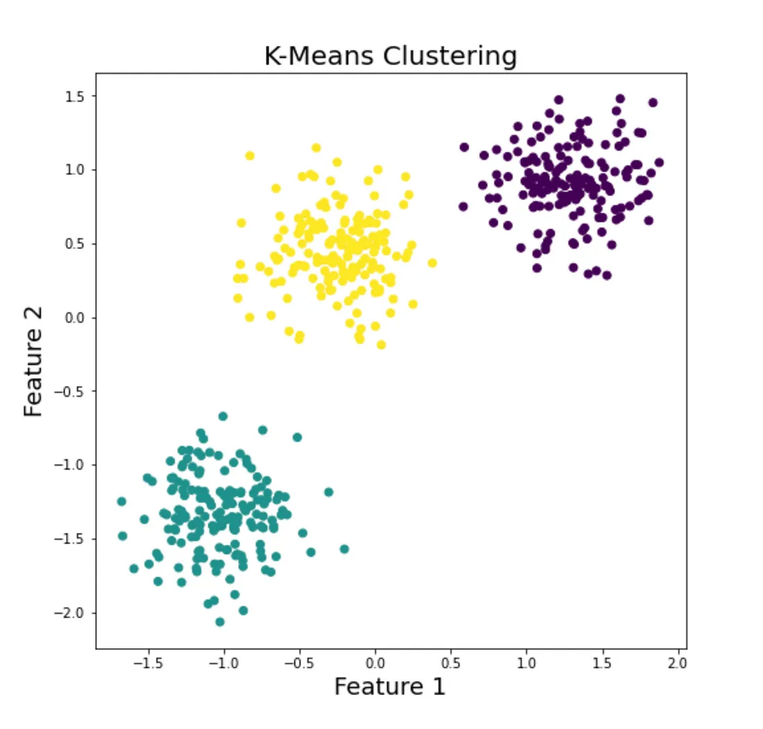
🧠 How It Works:

Initialize K centroids randomly.
Assign each data point to the nearest centroid.
Update centroids by calculating the mean of the assigned points.
Repeat until convergence (centroids no longer change).

🔍 Explore More:
Learn about K-Means in detail here.

b. Hands-On with K-Means

Get hands-on experience by implementing K-Means clustering in Python.

🔍 Follow Along with Code:
Check out this step-by-step tutorial on K-Means implementation here.

👾 DAY 3: Hierarchical Clustering

a. Hierarchical Clustering: Building Nested Clusters

Hierarchical clustering builds a hierarchy of clusters. It can be divided into Agglomerative (bottom-up approach) and Divisive (top-down approach) clustering.

🧠 How It Works:

Agglomerative: Start with each data point as a single cluster and merge the closest pairs iteratively until all points are in a single cluster.
Divisive: Start with one cluster containing all data points and recursively split it into smaller clusters.

🔍 Deep Dive:
Understand hierarchical clustering with this guide.

b. Visualizing Dendrograms

Dendrograms are tree-like diagrams that illustrate the arrangement of clusters produced by hierarchical clustering. They help to visualize the process and results of hierarchical clustering.

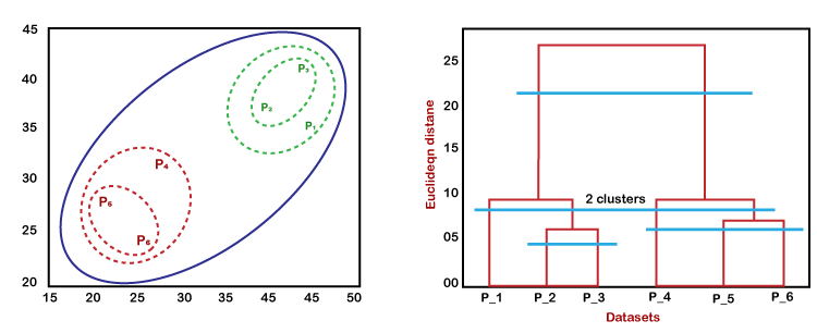
👾 DAY 4: Density-Based Clustering (DBSCAN)

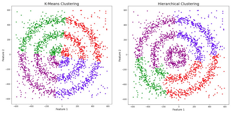
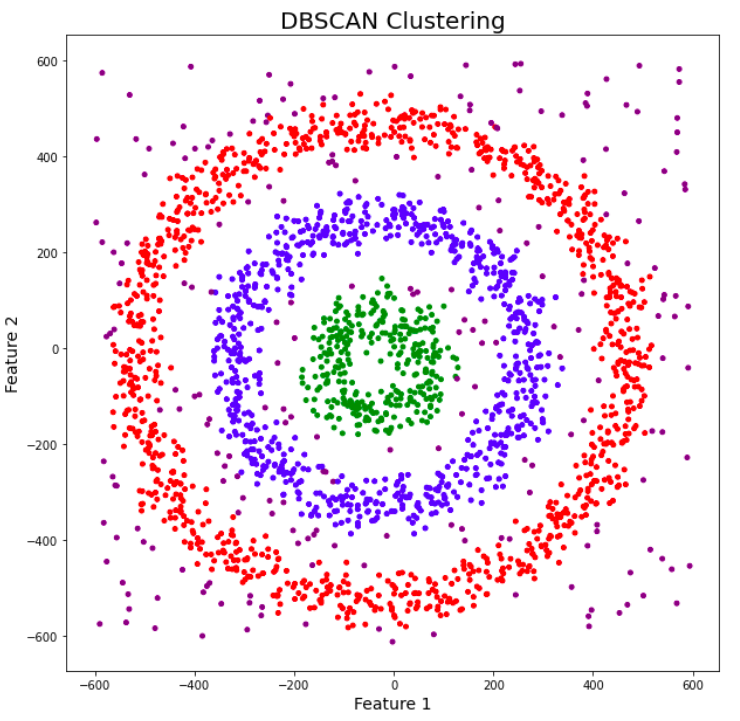
a. DBSCAN: Clustering Based on Density

Density-Based Spatial Clustering of Applications with Noise (DBSCAN) is a clustering algorithm that groups together points that are closely packed and marks points that are far away as outliers. It is particularly effective for datasets with noise and clusters of different shapes and sizes.

🧠 How It Works:

Select a point and find all points within a specified distance (epsilon).
If there are enough points (minimum samples), form a cluster.
Expand the cluster by repeating the process for each point in the cluster.
Mark points that don't belong to any cluster as noise.

🔍 Learn More:
Understand DBSCAN and its code in detail here.

b. Implementing DBSCAN

Get practical experience by implementing DBSCAN in Python.

🔍Take a look at the documentation:
You can go through the sklearn documentation for a better insight of DBSCAN.
https://scikit-learn.org/stable/auto_examples/cluster/plot_dbscan.html#sphx-glr-auto-examples-cluster-plot-dbscan-py

https://scikit-learn.org/stable/modules/generated/sklearn.cluster.DBSCAN.html

👾 DAY 5: Evaluation Metrics for Clustering

Clustering is only useful if we can evaluate the quality of the clusters it produces. This day will focus on understanding and using various metrics to assess clustering performance. These metrics help us determine how well our clustering algorithms are grouping similar data points and separating dissimilar ones.

a. Silhouette Score

Definition:
The silhouette score measures how similar an object is to its own cluster compared to other clusters. It ranges from -1 to 1, where a high value indicates that the object is well matched to its own cluster and poorly matched to neighboring clusters.

How It Works:

For each data point:
1. Calculate the average distance to all other points in the same cluster (a).
2. Calculate the average distance to all points in the nearest cluster (b).
3. The silhouette score for a point is given by:

\[ s = \frac{b - a}{\max(a, b)} \]

The overall silhouette score is the average of individual silhouette scores.

b. Davies-Bouldin Index

Definition:
The Davies-Bouldin Index (DBI) measures the average similarity ratio of each cluster with the cluster that is most similar to it. Lower DBI values indicate better clustering as they represent smaller within-cluster distances relative to between-cluster distances.

How It Works:

For each cluster:
1. Compute the average distance between each point in the cluster and the centroid of the cluster (within-cluster scatter).
2. Compute the distance between the centroids of the current cluster and all other clusters (between-cluster separation).
3. Calculate the DBI for each cluster and take the average.
4. The DBI is given by:
  \[ \text{DBI} = \frac{1}{N} \sum_{i=1}^{N} \max_{j \neq i} \left( \frac{s_i + s_j}{d_{ij}} \right) \]
  where s_i and s_j are the average distances within clusters (i) and (j), and (d_{ij}) is the distance between the centroids of clusters (i) and (j).

c. Adjusted Rand Index (ARI)

Definition:
The Adjusted Rand Index (ARI) measures the similarity between two clusterings by considering all pairs of samples and counting pairs that are assigned in the same or different clusters in the predicted and true clusterings. It adjusts for chance grouping.

How It Works:

Compute the Rand Index (RI):
1. Count pairs of points that are in the same or different clusters in both true and predicted clusters.
2. The RI is the ratio of the number of correctly assigned pairs to the total number of pairs.
Adjust the RI to account for chance clustering, resulting in ARI.

Formula:
\[ \text{ARI} = \frac{\text{RI} - \text{Expected\_RI}}{\max(\text{RI}) - \text{Expected\_RI}} \]

d. Practical Guide to Evaluating Clusters

Silhouette Analysis:
- When to Use: To determine the optimal number of clusters and understand cluster cohesion and separation.
- Practical Example: Implement silhouette analysis using Python’s scikit-learn library to evaluate K-means clustering results.
Davies-Bouldin Index:
- When to Use: To assess the quality of clustering where the clusters are of different shapes and sizes.
- Practical Example: Use the Davies-Bouldin Index to compare different clustering algorithms on a given dataset.
Adjusted Rand Index:
- When to Use: To compare the clustering results with ground truth labels.
- Practical Example: Compute the ARI to evaluate the clustering performance on a labeled dataset, such as customer segments with predefined categories.

🔍 Explore Metrics in Practice:
Explore the given metrices and its computation here.

e. Visualizing Clustering Results

Visualization is a powerful tool for interpreting and presenting clustering results. Common visualization techniques include:

Scatter plots: Useful for low-dimensional data, showing cluster assignments and centroids.
Heatmaps: Visualize distance matrices or similarity matrices.
Dendrograms: Illustrate the hierarchical clustering process.

👾 DAY 6: Dimensionality Reduction Techniques

Dimensionality reduction is crucial in unsupervised learning as it helps in simplifying models, reducing computation time, and mitigating the curse of dimensionality. This day will focus on understanding and applying different techniques for reducing the number of features in a dataset while preserving as much information as possible.

a. Principal Component Analysis (PCA)(Already discussed)

b. t-Distributed Stochastic Neighbor Embedding (t-SNE)

Definition:
t-SNE is a nonlinear technique for dimensionality reduction that is particularly well suited for visualizing high-dimensional datasets. It converts similarities between data points to joint probabilities and tries to minimize the Kullback-Leibler divergence between the joint probabilities of the low-dimensional embedding and the high-dimensional data.

How It Works:

Compute pairwise similarities in the high-dimensional space.
Define a probability distribution over pairs of high-dimensional objects.
Define a similar distribution over the points in the low-dimensional space.
Minimize the Kullback-Leibler divergence between these two distributions using gradient descent.

🔍 Learn More:
Understand the intricacies of t-SNE and its implementation here.

c. Linear Discriminant Analysis (LDA)

Definition:
LDA is a linear technique used for both classification and dimensionality reduction. It aims to find a linear combination of features that best separates two or more classes of objects or events. LDA is particularly useful when the data exhibits clear class separations.

How It Works:

Compute the mean vectors for each class.
Compute the scatter matrices (within-class scatter and between-class scatter).
Compute the eigenvalues and eigenvectors for the scatter matrices.
Select the top k eigenvectors to form a new matrix.
Transform the original data using this matrix to get the reduced dataset.

🔍 Learn More:
Dive deeper into LDA and its application here.

d. Uniform Manifold Approximation and Projection (UMAP)

Definition:
UMAP is a nonlinear dimensionality reduction technique that is based on manifold learning and is particularly effective for visualizing clusters in high-dimensional data. It constructs a high-dimensional graph of the data and then optimizes a low-dimensional graph to be as structurally similar as possible.

How It Works:

Construct a high-dimensional graph representation of the data.
Optimize a low-dimensional graph to preserve the topological structure.
Use stochastic gradient descent to minimize the cross-entropy between the high-dimensional and low-dimensional representations.

🔍 Learn More:
Learn about UMAP and its effectiveness in data visualization here.

e. Practical Guide to Dimensionality Reduction

Principal Component Analysis (PCA):
- When to Use: When you need to reduce dimensions linearly and want to preserve variance.
- Practical Example: Use PCA to reduce the dimensions of a dataset before clustering.
t-Distributed Stochastic Neighbor Embedding (t-SNE):
- When to Use: When you need to visualize high-dimensional data in 2 or 3 dimensions.
- Practical Example: Apply t-SNE to visualize customer segments in an e-commerce dataset.
Linear Discriminant Analysis (LDA):
- When to Use: When you need to perform dimensionality reduction for classification tasks.
- Practical Example: Use LDA to reduce the number of features in a labeled dataset before applying a classifier.
Uniform Manifold Approximation and Projection (UMAP):
- When to Use: When you need a fast and scalable way to visualize high-dimensional data.
- Practical Example: Employ UMAP to visualize clusters in genetic data.

🔍 Explore Techniques in Practice:
Learn how to apply these dimensionality reduction techniques using Python and real datasets in this comprehensive guide.

By the end of Day 6, you will have a thorough understanding of various dimensionality reduction techniques, how to implement them, and when to apply each method effectively. This knowledge will be crucial for handling high-dimensional data in unsupervised learning tasks. 🚀

👾 DAY 7: Practical Applications and Project Work

a. Applying Clustering to Real-World Data

Put your knowledge into practice by applying clustering algorithms to real-world datasets. This will solidify your understanding and help you tackle real-life problems.

🔍 Try It Out:
Explore practical clustering applications on kaggle.

b. Project: Customer Segmentation

Work on a project to segment customers based on their purchasing behavior. This project will help you understand how clustering can be used for market segmentation, personalized marketing, and more.

🔍 Follow Along with Project:
Check out this customer segmentation project here.

By following this week, you'll gain a strong foundation in clustering and unsupervised learning, empowering you to uncover hidden patterns and insights in your data. Happy clustering! 🚀

🦝 Week 8 and beyond (Projects, PyTorch)

TensorFlow Project

You will now do a project. You can make use of models available in keras. You would also need to use some pre-processing.

Go to this link, download the dataset and get working!

https://www.kaggle.com/datasets/mirichoi0218/insurance

P.S. some features aren't as useful as others, so you may want to use feature selection

https://www.javatpoint.com/feature-selection-techniques-in-machine-learning.

Don't worry if your results aren't that good, this isn't really a task to be done in 1 day. It's basically to give you hands-on experience. Also, there are notebooks available on kaggle for this problem given, you can take hints from there as well. There are many similar datasets available on kaggle, you can try those out too! Also, as you learn more topics in ML, you will get to know how to further improve accuracy. So just dive in and make a (working) model.

Some More Topics:

Following are some links which cover various techniques in ML. You may not need them all in this project, but you may need them in the future. Feel free to read and learn about them anytime, they are basically to help you build more efficient models and process the data more efficiently. Thus, you can cover these topics in the future as well.

https://machinelearningmastery.com/overfitting-and-underfitting-with-machine-learning-algorithms/

https://towardsdatascience.com/regularization-in-machine-learning-76441ddcf99a

https://towardsdatascience.com/train-validation-and-test-sets-72cb40cba9e7

https://machinelearningmastery.com/k-fold-cross-validation/

PyTorch

Additional Topics

Contributors

Anwesh Sen Saha | +91 84519 62003
Dhruv Singh | +91 96216 88942
Kartik Kulkarni | +91 91750 09924
Ridin Datta | +91 74390 79526
Talin Gupta | +91 85589 13121
Tejas Ahuja | +91 87007 94886