# Real Time Predictor of Hockey Match Outcomes
[University of Victoria](https://uvic.ca), Faculty of Engineering and Computer Science, Spring 2024
[SENG 474: Data Mining](https://www.uvic.ca/calendar/undergrad/#/courses/S1aylKTX4?q=seng474&&limit=20&skip=0&bc=true&bcCurrent=&bcCurrent=Data%20Mining&bcItemType=courses) final project. *Rough "page" count for grading reference: 24.*
By: [Matthew Trent](https://matthewtrent.me), [Mathew Terhune](https://github.com/mathewterhune), [Jack Barrett](https://github.com/barrettjack), and [Gabriel Maryshev](https://github.com/AcademicianZakharov).
<div style="text-align: center;">
<span>
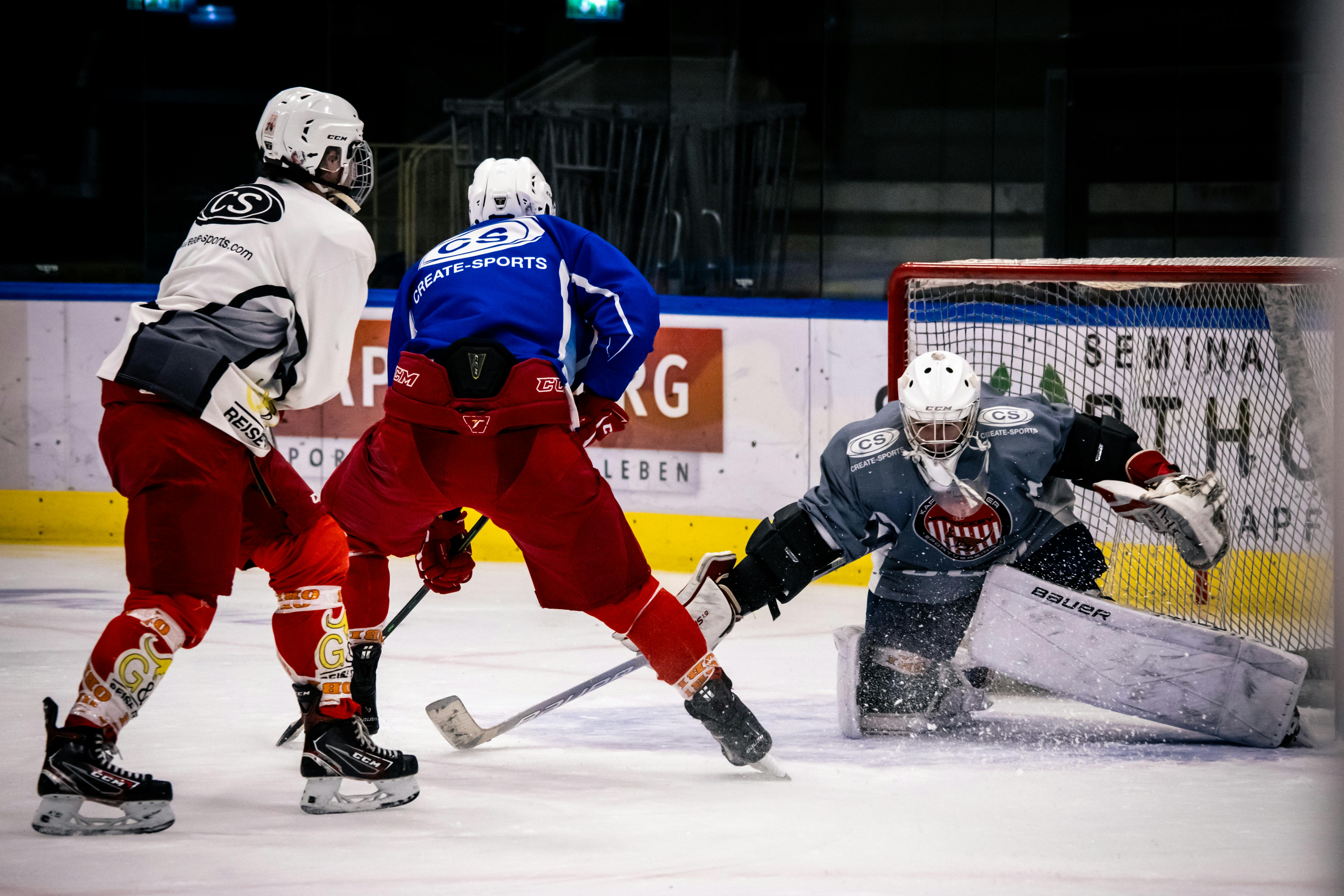
It's a goal! (via
<a target="_blank" href="https://www.pexels.com/photo/players-during-ice-hockey-game-19330475/">Pexels</a>)
</span>
</div>
---
## Abstract
This study presents a real-time predictor for hockey match outcomes, leveraging over 1.75 million shot entries from [MoneyPuck](https://moneypuck.com) to forecast game results as they unfold. We employed a unique combination of 42 specific and 2 engineered features to enhance our models' accuracy, precision, and recall. First, using logistic regression~3~, we devised a metric to assess each shot's quality, integrating this into our second model, a Long-Short Term Memory (LSTM)~1~ neural network, for dynamic game outcome prediction. This latter model's real-time capability sets it apart, providing valuable insights for commentators and spectators, contrasting with traditional pre-game or static in-game predictions. The results show that both our models outperform dummy classifiers, suggesting their potential utility in enhancing the live hockey viewing experience.
## Related work
There are a numerous platforms that offer a blend of sports statistics, analyses, and predictions. At a superficial level, our predictor may appear akin to others’: it accepts two teams as inputs and provides users with the likelihood of each winning as an output.
Our model differs in that are predicting the outcome of a game *in real time*, providing value to commentators and for spectators. This contrasts the typical use-case of the aforementioned models, whose primary utility is in providing insights for betting purposes.
Despite these differences, there are several notable platforms that engage in activities similar to ours:
- [MoneyPuck](https://moneypuck.com): This is a hockey-focused website that serves primarily as a repository for data, which also ventures into the realm of game predictions. Our initial dataset on shots was sourced from here. MoneyPuck leans more towards providing statistical data rather than facilitating betting.
- [Hockey Reference](https://websitesimilar.com/hockey-reference.com): This site is a comprehensive repository for hockey statistics, offering detailed information on players, teams, leagues, awards, records, leaders, rookies, and game scores.
## Introduction
In the evolving field of sports analytics, the use of data mining techniques has revolutionized our understanding and analysis of various sports, including hockey. This term project provides an in-depth exploration of how data mining techniques can be leveraged to forecast the outcomes of a hockey game, aiming to decipher the intricate patterns of a game, and offering predictions that could significantly benefit both teams and analysts.
The foundation of our research comes from the comprehensive shot dataset provided for free by [MoneyPuck](https://moneypuck.com), comprising over 1.75 million shot entries taken across games from 2007 to present. Each individual entry provides a surplus of information for our purposes, with 124 unique attributes. Thus, in our analysis, we elected to use 42 specific features, chosen for their relevance to our analysis, as well as 2 engineered features. This selective approach was chosen to enhance the precision, accuracy, and recall of our models.
The significance of this paper stems from the field of sports analytics. This area of research receives significant funding, and enables the acquisition of insights that, if leveraged, may yield competitive advantages for a hockey team; our motivation for this work is in part to provide insights of this kind.
## Dataset
Before introducing our dataset formally, we will provide context about its source. MoneyPuck, referenced beforehand in the introduction, is a website dedicated to the aggregation and maintenance of detailed statistics and analytics for the National Hockey League (NHL)~5~. Their data ranges from the 2008-2009 season to present, being updated daily in coincidence with live games.
For our purposes, they provide 2 free datasets of interest:
- Player biographical data: here, individual player statistics such as average shots-on-goal per game, average on-ice time per game, and so on, are detailed. Moreover, physical attributes such as height and weight are included. Data is provided for each season, and a unique key for each player is provided: ``player_id``.
- Shot level data: at over 1.7 million recorded shots, this dataset is a rich source of information. It captures every shot's specifics in great detail, providing 124 features per shot. To describe just three, we have features representing a shots location on the ice, the type of shot taken (e.g. a slap-shot), and finally the shooters angle from the net. In addition, we have ``shooter_id``, a foreign-key on the table above, and ``game_id``, which uniquely identifies those shots taken in a specific game.
The availability of the data on a per-season basis allowed us to significantly reduce the preprocessing and training time of our code and models; we elected to train and test our model on the 2022 data, as the data for this season alone contains over 1,000 games, amounting to over 100,000 rows of data. (Naturally, our model could be extended further by taking into consideration the remaining 16 years.)
## The process
### Overview
Below is an illustration with the x-axis (time) broken up into *n* partitions, with each new partition being created when a shot is taken. This axis comprises the entirety of a single hockey match. Then, on the y-axis (percent chance of each team winning), the values are discretely determined upon the advent of a new shot on the x-axis. Note that the summed y-axis values between both teams always obviously sum to 100%, creating an alluringly symmetrical graph.
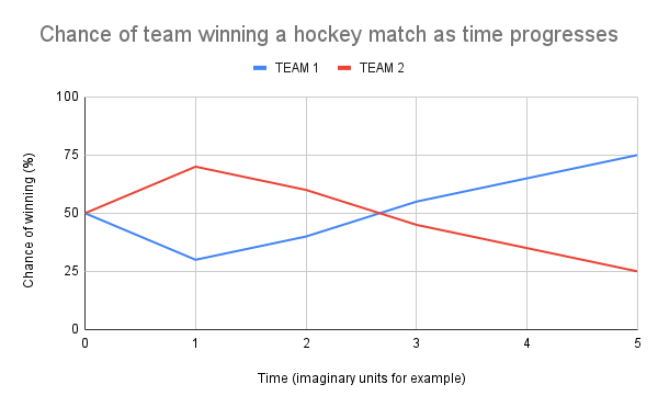
By first determining the quality of each shot and giving it a ranking; we could then feed each of the shots alongside this ranking into a neural net and hope that the quality of shots a team is taking during a game (even if they don't go in) predict their team's likelihood of winning.
### Step 1 of 4: Data mining
Before finalizing our approach, we explored a variety of methods, including:
1. Acquiring a `shots_<some_year>.csv` file from [MoneyPuck](https://moneypuck.com/data.htm) to get generic shots data.
2. Collecting information on individual players and their salaries through web scraping.
3. Web scraping player statistics (age, weight, height, etc.).
4. Utilizing a script to combine the two CSV files previously mentioned, akin to performing an SQL `JOIN` operation based on player names
5. Aggregating the newly formed CSV with each shot entry from the initial dataset by conducting an SQL-like JOIN operation, linking them through the player's ID, which is similar to their name
Ultimately, we discarded all of the above methods saving step one because they:
- Provided us too many columns to the point where we got minimum/negative returns.
- Caused us to remove many otherwise useful rows due to things like a player's data not existing in one of the CSVs we scraped.
Thus, we ended up using just the following shots data:
```py
# --- 2022 shots data ---
# shots is our pandas dataframe loaded with shots_2022.csv
shots.info()
# --- output ---
<class 'pandas.core.frame.DataFrame'>
RangeIndex: 122026 entries, 0 to 122025
Columns: 124 entries, shotID to yCordAdjusted
dtypes: float64(37), int64(74), object(13)
memory usage: 115.4+ MB
```
As seen above, this dataset had 124 unique columns, both of categorical and numerical nature. As one may guess, not all these rows were useful to us in our analyses:
```py
# --- numerical vs. categorical columns
print('numerical columns:', len(shots.select_dtypes(include=[np.number]).columns))
print('categorical columns:', len(shots.select_dtypes(include=[object]).columns))
# --- output ---
numerical columns: 111
categorical columns: 13
```
We utilized feature engineering to include an additional two columns, `shotType_shotDistance` and `shotAngle_shotDistance`, created like so:
```py
# --- feature engineering ---
# Adding engineered features (dividing one value by another)
shots['shotType_shotDistance'] = shots['timeSinceFaceoff'] / (shots['shotDistance'] + 1e-6) # no /0 errors
shots['shotAngle_shotDistance'] = shots['shotAngle'] / (shots['shotDistance'] + 1e-6) # no /0 errors
```
Additionally, it was important to acknowledge that MoneyPuck's datasets included their own shot predictions, indicated by columns prefixed with "x." To maintain the purity of our analysis, we opted to exclude these predictive metrics as they would influence our models outcomes.
```py
# --- removing predictive columns from the dataset ---
their_columns = [...]
their_columns_without_predictions = []
for f in their_columns:
if len(f) != 0 and f[0] != "x":
their_columns_without_predictions.append(f)
# original columns minus 9 predicted columns found and removed
print(their_columns_without_predictions)
```
In totality, we ended up using 45 columns features for our models, each of which can be explained in the data dictionary provided below.
#### Data dictionary
<details>
<summary><b>Click here</b> to expand the full data dictionary (features and their detailed descriptions).</summary>
<br>
| FeatureID | Feature Name | Feature Description |
|:--------- | ---------------------------------------------------- | --------------------------------------------------------------------------------------------------------------------- |
| 01 | `arenaAdjustedShotDistance` | The distance from where the shot was taken, adjusted to be suitable for all arenas. |
| 02 | `arenaAdjustedXCord` | The X-Coordinate on the ice from where the shot was taken, adjusted for arena idiosyncrasies. |
| 03 | `arenaAdjustedXCordABS` | The absolute value of the X-coordinate, providing distance from the center line, adjusted for arena differences. |
| 04 | `arenaAdjustedYCord` | The Y-Coordinate on the ice from where the shot was taken, adjusted for arena variations. |
| 05 | `arenaAdjustedYCordABS` | The absolute value of the Y-coordinate, indicating distance from a reference line, adjusted for the arena. |
| 06 | `averageRestDifference` | Possibly the average rest time difference between teams or players up to that point in the game. |
| 07 | `awayEmptyNet` | Indicates whether the away team's net is empty (goalie pulled) at the time of the shot. |
| 08 | `awayPenalty1Length` | The length of the first penalty assessed to the away team, likely active at the time of the shot. |
| 09 | `awayPenalty1TimeLeft` | Time remaining on the first active penalty against the away team. |
| 10 | `awaySkatersOnIce` | Number of away team skaters on the ice, which can vary due to penalties. |
| 11 | `defendingTeamAverageTimeOnIce` | Average time on ice for the defending team's players up to that point. |
| 12 | `defendingTeamAverageTimeOnIceOfDefencemen` | Average time on ice for the defending team's defensemen. |
| 13 | `defendingTeamAverageTimeOnIceOfDefencemenSinceFaceoff` | Average time on ice for the defending team's defensemen since the last faceoff. |
| 14 | `defendingTeamAverageTimeOnIceOfForwards` | Average time on ice for the defending team's forwards. |
| 15 | `defendingTeamAverageTimeOnIceOfForwardsSinceFaceoff` | Average time on ice for forwards since the last faceoff.|
| 16 | `defendingTeamAverageTimeOnIceSinceFaceoff` | Average time on ice for the defending team's players since the last faceoff. |
| 17 | `defendingTeamDefencemenOnIce` | Number of defensemen on the ice for the defending team. |
| 18 | `defendingTeamForwardsOnIce` | Number of forwards on the ice for the defending team. |
| 19 | `defendingTeamMaxTimeOnIce` | Maximum time on ice among all players of the defending team. |
| 20 | `defendingTeamMaxTimeOnIceOfDefencemen` | Maximum time on ice among the defending team's defensemen. |
| 21 | `defendingTeamMaxTimeOnIceOfDefencemenSinceFaceoff` | Max time on ice for defensemen since the last faceoff. |
| 22 | `defendingTeamMaxTimeOnIceOfForwards` | Maximum time on ice among the defending team's forwards. |
| 23 | `defendingTeamMaxTimeOnIceOfForwardsSinceFaceoff` | Max time on ice for forwards since the last faceoff. |
| 24 | `defendingTeamMaxTimeOnIceSinceFaceoff` | Maximum time on ice for any player since the last faceoff. |
| 25 | `defendingTeamMinTimeOnIce` | Minimum time on ice among all players of the defending team. |
| 26 | `defendingTeamMinTimeOnIceOfDefencemen` | Minimum time on ice among the defending team's defensemen. |
| 27 | `defendingTeamMinTimeOnIceOfDefencemenSinceFaceoff` | Min time on ice for defensemen since the last faceoff. |
| 28 | `defendingTeamMinTimeOnIceOfForwards` | Minimum time on ice among the defending team's forwards. |
| 29 | `defendingTeamMinTimeOnIceOfForwardsSinceFaceoff` | Min time on ice for forwards since the last faceoff. |
| 30 | `defendingTeamMinTimeOnIceSinceFaceoff` | Minimum time on ice for any player since the last faceoff. |
| 31 | `distanceFromLastEvent` | Distance from the location of the last event (like a pass or hit) to the shot. |
| 32 | `homeEmptyNet` | Indicates if the home team's net is empty at the time of the shot. |
| 33 | `homePenalty1Length` | Length of the first penalty against the home team. |
| 34 | `homePenalty1TimeLeft` | Time left on the first active penalty against the home team. |
| 35 | `homeSkatersOnIce` | Number of home team skaters on the ice. |
| 36 | `shotAngle` | The angle of the shot relative to the goal. |
| 37 | `shotDistance` | The distance from the shooter to the goal. |
| 38 | `shotType` | The type of shot (e.g., wrist shot, slap shot). |
| 39 | `speedFromLastEvent` | The speed of play from the last event to the shot. |
| 40 | `timeDifferenceSinceChange` | Time since the last line change or significant event. |
| 41 | `timeSinceFaceoff` | Time elapsed since the last faceoff. |
| 42 | `timeSinceLastEvent` | Time elapsed since the last recorded event in the game. |
| 43 | `timeUntilNextEvent` | Time until the next event after the shot. |
| 44 | `shotType_shotDistance` | |
| 45 | `shotAngle_shotDistance` | |
</details>
<br>
The histogram of our remaining features is as follows. Due to the sheer number of attributes we used, the titles aren't readable here, but it still stands to show rough correlations.
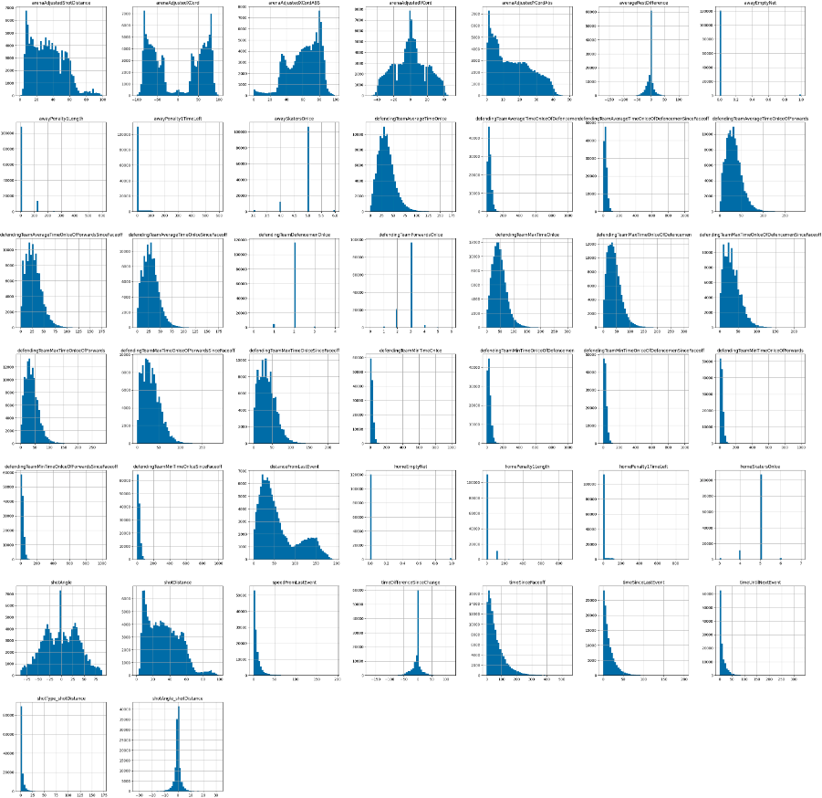
We used a similar histogram like this in great-depth with the initial feature set to determine features that had strong positive or negative correlations with the "goal" column.
### Step 2 of 4: Determining shot quality
The goal of this step was to create an algorithm that could do as follows:
```
input: shot row
output: a quality ranking between 0 and 1
example: shot ID 121 -> [ black box ] -> quality of 0.234122
```
We would then run it for all the rows in our dataset.
To accomplish this, we settled on using [logistic regression](https://en.wikipedia.org/wiki/Logistic_regression)~3~. This is a statistical machine learning algorithm that is used for binary classification that predicts the probability of a particular outcome occurring. For us, this outcome was *"will this shot result in a goal?"*.
To enumerate, we took a shot of the form below:
```py
i_th_shot_instance = [43.0, 47.0, 47.0, 8.0, 8.0, 0.0, 0, 0, 0, 5, 23.0, 23.0, 23.0, 23.0, 23.0, 23.0, 2, 3, 23, 23, 23, 23, 23, 23, 23, 23, 23, 23, 23, 23, 127.34598541, 0, 0, 0, 5, 10.0805979875, 45.7055795281, 'WRIST', 21.2243309016, 0, 23, 6, 1, 0.5032208263028077, 0.22055508038679]
```
Where each column mapped to one of the features we listed above in [step one](https://todo.com) and set our logistic regression~3~ model to classify it as a "good" (value closer to 1) shot if the model suspects a shot with its attributes would go in, and "bad" (closer to 0) if it thinks it would miss.
Our implementation used a pipeline as follows:
```py
pipeline = Pipeline([
# data processing
('preprocessing', ColumnTransformer([
('num', make_pipeline(
SimpleImputer(strategy='mean'),
PowerTransformer(),
MinMaxScaler()
), numerical_features),
('cat', OneHotEncoder(handle_unknown='ignore'), categorical_features)
])),
# later our model will include the argument "class_weight='balanced'"
# to fix an error discussed below
('classifier', LogisticRegression(max_iter=1000, random_state=42))
])
```
The `ColumnTransformer` in this pipeline allowed for us to apply many different functions to the data depending on if it was categorical or numeric in nature:
- Numerical data:
- `SimpleImputer`: Set any missing values to the mean of their column.
- `PowerTransformer`: Applied a power transformation to each feature, making the data more Guassian-like. This helped stabilize and balance skewness.
- `MinMaxScaler`: Scaled each feature to be between 0 and 1.
- Categorical data:
- `OneHotEncoder`: Transformed values into numerical representations. This is because logistic regression algorithms will not function properly with text input.
Finally, we ran our actual `LogisticRegression`~3~ model. Initially, it gave us an accuracy of 93% for predicting if a shot would go in or not given its attributes. However, we found that ~7% of all NHL shots go in and that 100% - 93% = 7% = our error percentage.
It turned out our predictor was overwhelmed by the existence of negative classes in our data. This meant it would predict "the shot will miss" indiscriminately and still be right 93% of the time. In machine learning, this sort of error is attributed to a "data imbalance".
> **Data imbalance**: Where your target variable's positive class ("if the shot went in") exists vastly more or vastly less than the negative class ("if the shot missed") in your dataset.
To fix this, we added the argument `class_weight='balanced'` to our `LogisticRegression` model.
```
ORIGINAL -> WITH BALANCED CLASS WEIGHT
---------- ----------------------------
Shot: goal goal
Shot: miss miss
Shot: miss miss
Shot: miss goal
Shot: miss miss
Shot: miss goal
Shot: miss goal
Shot: miss miss
Shot: miss goal
Shot: miss miss
```
This resulted in our data having a balanced representation between goals and misses, such that our model could no longer "cheat" by always predicting a miss.
With that done, we ran our model, and achieved fairly solid results:
```
model vs. dummy classifier:
accuracy - model: 0.89244 vs. dummy: 0.50299
recall - model: 0.97173 vs. dummy: 0.52106
precision - model: 0.40513 vs. dummy: 0.07701
F1 score - model: 0.57185 vs. dummy: 0.13419
predicting "quality" of each shot:
shot #1 "quality": 0.2446 - actual result: no goal
shot #2 "quality": 0.0022 - actual result: no goal
shot #3 "quality": 0.1028 - actual result: no goal
shot #4 "quality": 0.9164 - actual result: goal
shot #5 "quality": 0.3799 - actual result: no goal
shot #6 "quality": 0.0001 - actual result: no goal
shot #7 "quality": 0.0001 - actual result: no goal
shot #8 "quality": 0.0099 - actual result: no goal
shot #9 "quality": 0.7397 - actual result: no goal
shot #10 "quality": 0.0253 - actual result: no goal
... etc.
```
As shown above, a high "quality" score prediction from our model results in an actual goal being scored.
To summarize the accuracy, recall, precision, and F1 scores from this output, our model:
- Identified goals correctly 97% of the time.
- Of the "is a goal" predictions, 40% were actually goals.
- It was good at "getting all the goals", but had a fair amount of false positives.
- Beat the dummy classifier where it needed to.
To us, this was a fine result, as we wanted our neural net to ultimately decide on the threshold for a shot's "quality" that resulted it in being classified as a goal. For the above example, we simply used 0.5 as a stand-in.
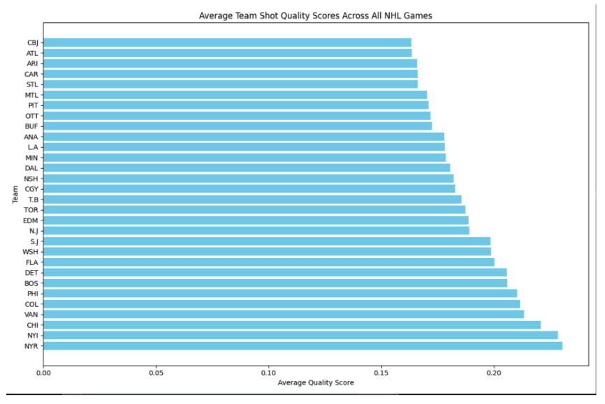
As an aside, we found an interesting relation between shot quality and teams. However, it does not exactly map to anything meaningful, such as the [Stanley Cup](https://en.wikipedia.org/wiki/Stanley_Cup)~5~ ranking for said season. We assume this is because a team's overall ability to do well is comprised of too many variables therefore attempting to derive an order from just their average shot quality is too naive of an approach.
### Step 3 of 4: Preprocessing shot quality for the neural net
Next, we needed to find a way to properly bundle the data from each individual hockey match with its associated shots and our matching quality metrics for each shot, so that we could feed them as input to the neural net.
Moreover, we figured we could throw in some additional attributes that we had access to before, but didn't previously make sense to include when we were only predicting the quality of a single shot.
Our goal was to build an algorithm that could do the following:
```
input: entire shots dataset
output: JSON data grouped by game, including sequential shots data and
additional metadata
example: shot_2022.csv -> [ black box ] -> [{'game_id': 21223, ...}, ...]
```
To achieve this, our black box implementation looked as follows:
```py
# games summary array
games_summary = []
# get all the unique game_ids from the shots data set
game_ids = shots['game_id'].unique()
# loop through each game_id
for gid in game_ids:
# get all the shots for the current game
game_shots = shots[shots['game_id'] == gid]
# get the two teams playing in the game
teams = [game_shots['homeTeamCode'].iloc[0], game_shots['awayTeamCode'].iloc[0]]
if len(teams) != 2:
print(f"warning: not exactly two teams identified for game {gid}, check the data for accuracy")
continue
# initialize the game summary dictionary
game_summary = {
"game_id": gid,
"overall_score": {},
"shots_by_time": []
}
# initialize score for both teams
score = {team: 0 for team in teams}
# initialize a dictionary to track the number of shots per player
player_shots_count = {}
# loop through each shot in the game
for index, row in game_shots.iterrows():
team_code = row['teamCode']
shooter_name = row['shooterName']
# update the shot count for this player
if shooter_name in player_shots_count:
player_shots_count[shooter_name] += 1
else:
player_shots_count[shooter_name] = 1 # first shot for this player
# if the shot was a goal, update the score for this game
if row['goal'] == 1:
score[team_code] += 1
# calculate "goodness" of the shot using our earlier model
shot_features = row[features].to_frame().T
goodness_score = pipeline.predict_proba(shot_features)[0][1] # get the probability of the positive class
# append shot data including the "goodness" score and player's shot number
game_summary['shots_by_time'].append({
"team_taking_shot": team_code,
"shooter_name": shooter_name,
"players_shot_n": player_shots_count[shooter_name], # include the shot number for this player
"goal": row['goal'] == 1,
"score_at_this_point": score.copy(),
"quality": goodness_score
})
game_summary['overall_score'] = score
games_summary.append(game_summary)
# print the summary of the first game for demonstration
if games_summary: # checking if the list is not empty
print(games_summary[0])
```
This output an *n*-length array where each element was of the form below highlighting the results from a specific game. Internally, its`shots_by_time` array would be of *m*-length, where *m* is the number of shots in that game. This example output is intentionally shortened to a single game with only a few shots.
```json
{
"game_id": 20001,
"overall_score": {
"NSH": 4,
"SJS": 1
},
"shots_by_time": [
{
"team_taking_shot": "SJS",
"shooter_name": "Timo Meier",
"players_shot_n": 1,
"goal": false,
"score_at_this_point": {
"NSH": 0,
"SJS": 0
},
"quality": 0.23172020145933714
},
{
"team_taking_shot": "SJS",
"shooter_name": "Marc-Edouard Vlasic",
"players_shot_n": 1,
"goal": false,
"score_at_this_point": {
"NSH": 0,
"SJS": 0
},
"quality": 0.002285905055888781
},
{
"team_taking_shot": "NSH",
"shooter_name": "Mattias Ekholm",
"players_shot_n": 1,
"goal": false,
"score_at_this_point": {
"NSH": 0,
"SJS": 0
},
"quality": 0.0983513158171244
},
{
"team_taking_shot": "NSH",
"shooter_name": "Kiefer Sherwood",
"players_shot_n": 1,
"goal": true,
"score_at_this_point": {
"NSH": 1,
"SJS": 0
},
"quality": 0.912882665282009
}
]
}
```
The meaning behind this data structure is as follows:
| Key | Description |
|-----------------------|-----------------------------------------------------------------------------------------------------|
| `game_id` | Unique identifier for the game. |
| `overall_score` | Dictionary containing the final scores for the teams, with team abbreviations as keys. |
| `shots_by_time` | An array of shot events, each with details about the shot. |
The `shots_by_time` array takes the form of *m* shots that partition the game ordered sequentially by time of shot, with the earliest shot coming fist:
| Key | Description |
|-----------------------|-----------------------------------------------------------------------------------------------------|
| `team_taking_shot` | Abbreviation of the team that took the shot. |
| `shooter_name` | Name of the player who took the shot. |
| `players_shot_n` | How many shots this particular player has taken so far this game. |
| `goal` | Boolean indicating whether the shot resulted in a goal (`true`) or not (`false`). |
| `score_at_this_point` | Dictionary showing the score of both teams at the time of this shot. |
| `quality` | A shot's quality. This comes directly from our original logistic regression. |
### Step 4 of 4: Real time game prediction
> **Long-Short Term Memory**: LSTM~1~ networks are a specialized type of recurrent neural network~8~ used in deep learning for tasks that are based on sequential data. These networks are excellent at classification, processing, and predictive outcomes of on a series of inputs. Some notable applications of these models include, language modeling and text generation, speech recognition, and anomaly detection, and much more. A key strength of Long-Short term memory networks is their ability to address the issue of long term dependencies, which is relevant in recurrent neural networks. This capability is crucial in sequence processing tasks where it's important to retain information from initial steps and leverage it in subsequent stages of the sequence.
**Implementation of the LSTM~1~**
```python
import pandas as pd
import numpy as np
from tensorflow.keras.models import Sequential
from tensorflow.keras.layers import LSTM, Dense, Dropout
from sklearn.preprocessing import MinMaxScaler
from tensorflow.keras import regularizers
# Load the dataset
df = pd.read_csv('./shots.csv')
chunksize = 10000
# Read the data in chunks
for chunk in pd.read_csv('./shots.csv', chunksize=chunksize):
# Preprocess the data
features = ['homeTeamGoals', 'awayTeamGoals',
'shootingTeamForwardsOnIce', 'shootingTeamDefencemenOnIce', 'defendingTeamForwardsOnIce',
'defendingTeamDefencemenOnIce']
X = chunk[features].values
y = chunk['homeTeamWon'].values
# Split the data into sequences
sequence_length = 10 # Number of shots to consider
X = np.array([X[i:i+sequence_length] for i in range(len(X)-sequence_length)])
y = y[sequence_length:]
# Normalize the data
scaler = MinMaxScaler()
X = scaler.fit_transform(X.reshape(-1, X.shape[-1])).reshape(X.shape)
# Split the data into training and testing sets
split_index = int(0.8 * len(X))
X_train, X_test = X[:split_index], X[split_index:]
y_train, y_test = y[:split_index], y[split_index:]
# Build the LSTM model
model = Sequential()
model.add(LSTM(64, input_shape=(sequence_length, len(features))))
model.add(Dropout(0.3))
model.add(Dense(64, activation='relu', kernel_regularizer=regularizers.l2(0.02)))
model.add(Dense(32, activation='relu'))
model.add(Dropout(0.2))
model.add(Dense(1, activation='sigmoid'))
# Compile the model
model.compile(optimizer='adam', loss='binary_crossentropy', metrics=['accuracy'])
# Train the model
model.fit(X_train, y_train, epochs=15, batch_size=32, validation_data=(X_test, y_test))
# Evaluate the model
loss, accuracy = model.evaluate(X_test, y_test)
print(f'Test accuracy: {accuracy:.4f}')
# Make predictions
prev_game_id = None
not_first_game = False
count = 0
for i in range(len(X_test)):
sequence = X_test[i]
prediction = model.predict(np.expand_dims(sequence, axis=0), verbose = 0)[0][0]
game_id = chunk['game_id'].iloc[i + split_index + sequence_length - 1]
if game_id != prev_game_id:
if not_first_game and count > 1:
print(f"Results of game: {prev_game_id}, home team score:{chunk['homeTeamGoals'].iloc[i+ split_index+ sequence_length -2]}, away team score:{chunk['awayTeamGoals'].iloc[i + split_index + sequence_length -2]}")
print("----------------------------------------------------------------------------------------------------")
prev_game_id = game_id
if count > 0:
print(f"New game: {game_id}, home team score:{chunk['homeTeamGoals'].iloc[i + split_index + sequence_length -1]}, away team score:{chunk['awayTeamGoals'].iloc[i + split_index + sequence_length-1]}")
count += 1
not_first_game = True
if count > 1:
if i % 10 == 0:
home_team_score = chunk['homeTeamGoals'].iloc[i + split_index + sequence_length -1]
away_team_score = chunk['awayTeamGoals'].iloc[i + split_index + sequence_length -1]
if home_team_score+away_team_score > 0:
print(f'Probability of home team winning after {sequence_length} shots: {prediction:.2f}, dummy classifier score: = {home_team_score/(home_team_score+away_team_score)}')
```
The neural network uses a sliding window of 10 shots to predict if the home team will win.
**Sample output after 15 epochs of training**
```
Epoch 15/15
250/250 ━━━━━━━━━━━━━━━━━━━━ 2s 6ms/step - accuracy: 0.7052 - loss: 0.5477 - precision: 0.7228 - recall: 0.8082 - val_accuracy: 0.7152 - val_loss: 0.5384 - val_precision: 0.6868 - val_recall: 0.8542
63/63 ━━━━━━━━━━━━━━━━━━━━ 0s 3ms/step - accuracy: 0.7336 - loss: 0.5470 - precision: 0.7836 - recall: 0.8009
Test accuracy: 0.7152, Test precision: 0.6868, Test recall: 0.8542,
New game: 20094, home team score:0, away team score:0
Probability of home team winning after 10 shots: 0.61, dummy classifier score: = 1.0
Probability of home team winning after 10 shots: 0.48, dummy classifier score: = 0.5
Probability of home team winning after 10 shots: 0.37, dummy classifier score: = 0.3333333333333333
Probability of home team winning after 10 shots: 0.28, dummy classifier score: = 0.25
Probability of home team winning after 10 shots: 0.24, dummy classifier score: = 0.4
Probability of home team winning after 10 shots: 0.13, dummy classifier score: = 0.4
Probability of home team winning after 10 shots: 0.53, dummy classifier score: = 0.5
Probability of home team winning after 10 shots: 0.96, dummy classifier score: = 0.625
Probability of home team winning after 10 shots: 0.95, dummy classifier score: = 0.625
Probability of home team winning after 10 shots: 0.95, dummy classifier score: = 0.625
Results of game: 20094, home team score:6, away team score:3
----------------------------------------------------------------------------------------------------
New game: 20095, home team score:0, away team score:0
Probability of home team winning after 10 shots: 0.61, dummy classifier score: = 1.0
Probability of home team winning after 10 shots: 0.66, dummy classifier score: = 1.0
Probability of home team winning after 10 shots: 0.63, dummy classifier score: = 1.0
Probability of home team winning after 10 shots: 0.63, dummy classifier score: = 1.0
Probability of home team winning after 10 shots: 0.93, dummy classifier score: = 1.0
Results of game: 20095, home team score:3, away team score:0
----------------------------------------------------------------------------------------------------
New game: 20096, home team score:0, away team score:0
Probability of home team winning after 10 shots: 0.67, dummy classifier score: = 1.0
Probability of home team winning after 10 shots: 0.74, dummy classifier score: = 1.0
Probability of home team winning after 10 shots: 0.63, dummy classifier score: = 1.0
Probability of home team winning after 10 shots: 0.64, dummy classifier score: = 0.5
Probability of home team winning after 10 shots: 0.56, dummy classifier score: = 0.5
Probability of home team winning after 10 shots: 0.83, dummy classifier score: = 0.6666666666666666
Probability of home team winning after 10 shots: 0.94, dummy classifier score: = 0.75
Results of game: 20096, home team score:3, away team score:1
----------------------------------------------------------------------------------------------------
New game: 20097, home team score:0, away team score:0
Probability of home team winning after 10 shots: 0.50, dummy classifier score: = 0.0
Probability of home team winning after 10 shots: 0.61, dummy classifier score: = 0.5
Probability of home team winning after 10 shots: 0.59, dummy classifier score: = 0.5
Probability of home team winning after 10 shots: 0.58, dummy classifier score: = 0.5
Probability of home team winning after 10 shots: 0.56, dummy classifier score: = 0.5
Probability of home team winning after 10 shots: 0.17, dummy classifier score: = 0.25
Probability of home team winning after 10 shots: 0.27, dummy classifier score: = 0.4
Results of game: 20097, home team score:2, away team score:3
----------------------------------------------------------------------------------------------------
New game: 20098, home team score:0, away team score:0
Probability of home team winning after 10 shots: 0.45, dummy classifier score: = 0.0
Probability of home team winning after 10 shots: 0.41, dummy classifier score: = 0.0
Probability of home team winning after 10 shots: 0.37, dummy classifier score: = 0.0
Probability of home team winning after 10 shots: 0.19, dummy classifier score: = 0.0
Probability of home team winning after 10 shots: 0.06, dummy classifier score: = 0.0
Probability of home team winning after 10 shots: 0.02, dummy classifier score: = 0.16666666666666666
Probability of home team winning after 10 shots: 0.03, dummy classifier score: = 0.2857142857142857
Results of game: 20098, home team score:2, away team score:6
----------------------------------------------------------------------------------------------------
New game: 20100, home team score:0, away team score:0
Probability of home team winning after 10 shots: 0.60, dummy classifier score: = 1.0
Probability of home team winning after 10 shots: 0.48, dummy classifier score: = 0.5
Probability of home team winning after 10 shots: 0.56, dummy classifier score: = 0.5
Probability of home team winning after 10 shots: 0.79, dummy classifier score: = 0.6666666666666666
Probability of home team winning after 10 shots: 0.81, dummy classifier score: = 0.6666666666666666
Probability of home team winning after 10 shots: 0.88, dummy classifier score: = 0.75
Results of game: 20100, home team score:3, away team score:1
----------------------------------------------------------------------------------------------------
New game: 20101, home team score:0, away team score:0
Probability of home team winning after 10 shots: 0.47, dummy classifier score: = 0.0
Probability of home team winning after 10 shots: 0.49, dummy classifier score: = 0.0
Probability of home team winning after 10 shots: 0.72, dummy classifier score: = 0.5
Probability of home team winning after 10 shots: 0.74, dummy classifier score: = 0.5
Probability of home team winning after 10 shots: 0.27, dummy classifier score: = 0.3333333333333333
Probability of home team winning after 10 shots: 0.38, dummy classifier score: = 0.3333333333333333
Probability of home team winning after 10 shots: 0.41, dummy classifier score: = 0.3333333333333333
Results of game: 20101, home team score:1, away team score:3
----------------------------------------------------------------------------------------------------
New game: 20102, home team score:0, away team score:0
Probability of home team winning after 10 shots: 0.64, dummy classifier score: = 1.0
Probability of home team winning after 10 shots: 0.48, dummy classifier score: = 0.5
Probability of home team winning after 10 shots: 0.24, dummy classifier score: = 0.25
Probability of home team winning after 10 shots: 0.07, dummy classifier score: = 0.2
Probability of home team winning after 10 shots: 0.07, dummy classifier score: = 0.2
Probability of home team winning after 10 shots: 0.07, dummy classifier score: = 0.2
Probability of home team winning after 10 shots: 0.07, dummy classifier score: = 0.3333333333333333
Probability of home team winning after 10 shots: 0.05, dummy classifier score: = 0.25
Results of game: 20102, home team score:2, away team score:6
```
### Dummy classifier
```python=
import pandas as pd
import numpy as np
from sklearn.preprocessing import MinMaxScaler
from sklearn.metrics import accuracy_score, precision_score, recall_score
# Load the dataset
df = pd.read_csv('./shots.csv')
chunksize = 10000
# Initialize variables to accumulate results
dummy_accuracies = []
dummy_precisions = []
dummy_recalls = []
# Read and process the data in chunks
for chunk in pd.read_csv('./shots.csv', chunksize=chunksize):
# Preprocess the data
features = ['homeTeamGoals', 'awayTeamGoals',
'shootingTeamForwardsOnIce', 'shootingTeamDefencemenOnIce', 'defendingTeamForwardsOnIce',
'defendingTeamDefencemenOnIce']
X = chunk[features].values
y = chunk['homeTeamWon'].values
# Split the data into sequences
sequence_length = 10 # Number of shots to consider
X = np.array([X[i:i+sequence_length] for i in range(len(X)-sequence_length)])
y = y[sequence_length:]
# Normalize the data
scaler = MinMaxScaler()
X = scaler.fit_transform(X.reshape(-1, X.shape[-1])).reshape(X.shape)
# Split the data into training and testing sets
split_index = int(0.8 * len(X))
X_test = X[split_index:]
y_test = y[split_index:]
# Create dummy predictions
dummy_predictions = []
for i in range(len(X_test)):
home_team_goals = chunk['homeTeamGoals'].iloc[i + split_index + sequence_length - 1]
away_team_goals = chunk['awayTeamGoals'].iloc[i + split_index + sequence_length - 1]
total_goals = home_team_goals + away_team_goals
prediction = 1 if total_goals > 0 and home_team_goals / total_goals > 0.5 else 0
dummy_predictions.append(prediction)
# Adjusting y_test for length
y_test_adjusted = y_test[:len(dummy_predictions)]
# Calculate accuracy, precision, and recall for dummy classifier
accuracy = accuracy_score(y_test_adjusted, dummy_predictions)
precision = precision_score(y_test_adjusted, dummy_predictions)
recall = recall_score(y_test_adjusted, dummy_predictions)
# Accumulate results
dummy_accuracies.append(accuracy)
dummy_precisions.append(precision)
dummy_recalls.append(recall)
# Average the results across all chunks
average_accuracy = np.mean(dummy_accuracies)
average_precision = np.mean(dummy_precisions)
average_recall = np.mean(dummy_recalls)
print(f'{average_accuracy}, {average_precision}, {average_recall}')
```
(0.6925012153852067, 0.8308680371874702, 0.5320594866969488)
## Evaluation
The dummy classifier is simply using the score of the home team / total score as a probability of the home team winning. The LSTM~1~ neural network tends to overfit the data with more epochs, however after adding L2 regularization~7~, it was able to penalize large weights on some features thus achieving a higher accuracy on the test set.
In the test set evaluation, the LSTM~1~ model displayed higher accuracy (0.7152) and significantly better recall (0.8542) but lower precision (0.6868) compared to the dummy classifier, which showed an accuracy of 0.6925, precision of 0.8309, and recall of 0.5321.
Striving for a significantly higher accuracy than the dummy classifier might not be overly beneficial, as the primary features used by the LSTM~1~ are `homeTeamsGoals` and `awayTeamGoals`. Given their substantial influence, the LSTM~1~ is only going to have slightly better performance than a dummy classifier. Other contributing factors like `shootingTeamForwardsOnIce`, `shootingTeamDefencemenOnIce`, `defendingTeamForwardsOnIce`, and `defendingTeamDefencemenOnIce` have a relatively minor impact on determining the winning team.`1`
Moreover, the inclusion of additional features in the LSTM~1~ often results in overfitting the training data. This is somewhat expected because the supplementary features available in the NHL~6~ shots dataset are mainly related to shots, which do not promise significant model improvements. Hence, the decision was made not to incorporate shot quality as a feature to avoid exacerbating the overfitting issue.
While the current dataset is centered around shot data, introducing elements like "time of puck control" or "number of passes" could enable the LSTM~1~ to significantly outdo the dummy classifier. Nevertheless, it's important to note that the LSTM~1~ generates smoother outputs than the dummy classifier. This quality makes the LSTM~1~ particularly suitable for real-time game predictions, serving spectators and commentators with an AI that provides ongoing and fluid game insights.
## Conclusion
We created a shot quality metric via logistic regression and then trained an LSTM~1~ to predict the winning team in real time using a dataset of 1.75 million shots. As demonstrated by our analysis, our models outperform the dummy classifiers. In particular, we posit that their utility lies in the enhancement of the live hockey viewing experience by providing real-time game odds, and in revealing the essential characteristics of high-quality shots. Nevertheless, our models have limitations and more work would be needed for them to be more performant. Even though adding more features to the current model leads to overfitting, adding more significant features such as a feature that we do not have, like "control over puck" could potentially improve the models performance. Moreover, exploring whether the addition of player specific data on a per-shot basis provides positive predictive utility is a natural avenue to explore. Fine-tuning the dropout rate and the L2 regularization~7~ could also increase the LSTM~1~'s performance.
## Glossary
| ID | Term | Description |
|----|------------------------------|----------------|
| 1 | Long-Short Term Memory (LSTM) | A type of recurrent neural network (RNN) architecture used in the field of deep learning. |
| 2 | Deep learning | A subset of machine learning involving neural networks with multiple layers, capable of discovering representations from data without manual feature injection. |
| 3 | Logistic Regression | A statistical machine learning algorithm used for binary classification that predicts the probability of a particular outcome occurring. |
| 4 | Shot Quality | The quality of a shot generated from our logistic regression model, resulting in a "quality" of an individual shot. |
| 5 | Stanley Cup | The Stanley Cup is the championship trophy awarded annually to the National Hockey League (NHL) playo ff winner. |
| 6 | NHL | National Hockey League. |
| 7 | L2 Regularization | A technique used in machine learning to prevent overfitting. |
| 8 | Recurrent Neural Network |An RNN is a neural network that processes sequences, using its memory to retain information from previous inputs. |
## Acknowledgements
We thank [Dr. Alex Thomo](https://webhome.cs.uvic.ca/~thomo/) for his guidance throughout this course and project. We all learned so much!
 Sign in with Wallet


