## Beyond OpenMP and MPI: GPU parallelisation
### 5.1 Welcome to Week 5
In this week we will go beyond classical parallelisation paradigms (like OpenMP and MPI) which are generally associated with CPUs. We will talk about Graphics Processing Units (GPUs) that were originally developed for executing graphical tasks (including rendering in computer games) but can also be used for general-purpose computing in many fields.
We have already introduced GPUs in the first week. Through the steps of this week we will give some more details. We shall present the architecture of modern GPUs and then the available GPU execution models for computing acceleration. OpenMP as a means for "off-loading" parallel tasks to GPUs will be shortly introduced, while the main focus will be dedicated to two extensions to C for programming GPUs: CUDA and OpenCL. On one hand, directive-based GPU off-loading is simple to use but it's quite limited, contrary to GPU programming which requires more effort but offers more flexibility. Hopefully, the provided hands-on examples will introduce you to the topic of GPU programming as smoothly as possible.
### 5.2 GPU Architecture
To better understand the capabilities of GPUs in terms of computing acceleration, we will have a look at a typical architecture of a modern GPU.
As we already pointed out, GPUs were originally designed to accelerate graphics. They excel at operations (such as shading and rendering) on graphical primitives which constitute a 3D graphical object. The main characteristic of these primitives is that they are independent or, in other words, they can be processed independently in a parallel fashion. Thus, GPU acceleration of graphics was designed for the execution of inherently parallel tasks. On the other hand, CPUs are designed to execute the workflow of any general-purpose program, where many parallel tasks may not be involved. These different design principles reflect the fact that GPUs have many more processing units and higher memory bandwidth, while CPUs are characterized by more specialized processing of instructions and faster clock speed rates.
In the image below you can observe schematics of both CPU and GPU hardware architectures. From the schematics it is evident that:
- a GPU has many more arithmetic logic units or ALUs (green rectangles) than a CPU;
- a GPU can control simple, highly parallel workloads well (there's a yellow rectangle for every row of green rectangles), contrary to a CPU which can control more complex workloads;
- a core (green rectangle) in a CPU is different than a "core" or ALU (green rectangle) in a GPU: the former is comprised of ALUs and FPUs which are more specialized than ALUs in a GPU;
- a CPU has more cache memory than a GPU.
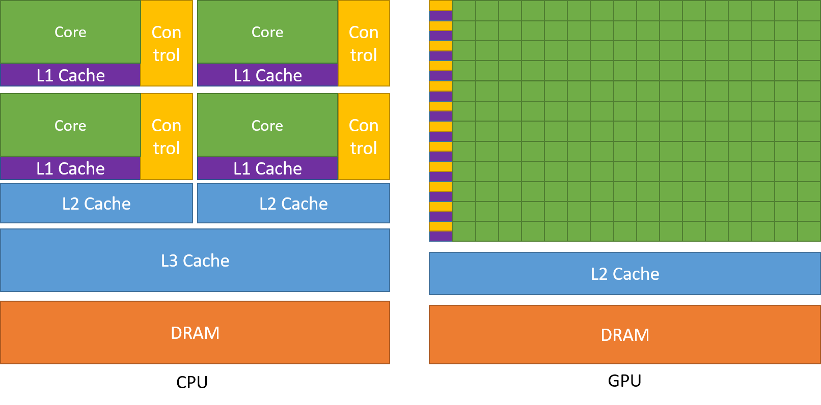
**Source of image: nvidia.com**
Note that the term "GPU core" is more or less a marketing term. The equivalent of a CPU core in a GPU is a streaming multiprocessor (SM) with many ALUs or "cores" (typically more than 100). Each SM has a lot of (L1 cache) registers (32-64 KB), instruction scheduler dispatchers and a very fast shared memory. In the next step we will put everything explained so far into perspective by showing some numbers.
See also:
[GPU architecture](https://docs.nvidia.com/cuda/cuda-c-programming-guide/index.html#from-graphics-processing-to-general-purpose-parallel-computing__gpu-devotes-more-transistors-to-data-processing)
### 5.3 GPUs by numbers
Desktop PCs or laptops are standardly equipped with a GPU, either integrated or as a standalone card. But how do such GPUs differ from GPUs dedicated to computing, e.g., on supercomputers (HPC clusters)?
First, let's have a look at the GPUs that are installed on the *Marconi-100* cluster (currently #18 on the [Top500 list](https://www.top500.org/lists/top500/list/2021/11/) of supercomputers in the world). By invoking the diagnostic utilities `deviceQuery` and `bandwidthTest` in the terminal of the login node we can get:
Output (excerpt) from `deviceQuery`:
```
Detected 4 CUDA Capable device(s)
Device 0: "Tesla V100-SXM2-16GB"
CUDA Driver Version / Runtime Version 11.0 / 10.2
CUDA Capability Major/Minor version number: 7.0
Total amount of global memory: 16128 MBytes (16911433728 bytes)
(80) Multiprocessors, ( 64) CUDA Cores/MP: 5120 CUDA Cores
GPU Max Clock rate: 1530 MHz (1.53 GHz)
Memory Clock rate: 877 Mhz
Memory Bus Width: 4096-bit
L2 Cache Size: 6291456 bytes
Maximum Texture Dimension Size (x,y,z) 1D=(131072), 2D=(131072, 65536), 3D=(16384, 16384, 16384)
Maximum Layered 1D Texture Size, (num) layers 1D=(32768), 2048 layers
Maximum Layered 2D Texture Size, (num) layers 2D=(32768, 32768), 2048 layers
Total amount of constant memory: 65536 bytes
Total amount of shared memory per block: 49152 bytes
Total number of registers available per block: 65536
Warp size: 32
Maximum number of threads per multiprocessor: 2048
Maximum number of threads per block: 1024
Max dimension size of a thread block (x,y,z): (1024, 1024, 64)
Max dimension size of a grid size (x,y,z): (2147483647, 65535, 65535)
Maximum memory pitch: 2147483647 bytes
Texture alignment: 512 bytes
Concurrent copy and kernel execution: Yes with 4 copy engine(s)
Run time limit on kernels: No
Integrated GPU sharing Host Memory: No
Support host page-locked memory mapping: Yes
Alignment requirement for Surfaces: Yes
Device has ECC support: Enabled
Device supports Unified Addressing (UVA): Yes
Device supports Compute Preemption: Yes
Supports Cooperative Kernel Launch: Yes
Supports MultiDevice Co-op Kernel Launch: Yes
Device PCI Domain ID / Bus ID / location ID: 4 / 4 / 0
```
Output (excerpt) from `bandwidthTest`:
```
Device 0: Tesla V100-SXM2-16GB
Quick Mode
Host to Device Bandwidth, 1 Device(s)
PINNED Memory Transfers
Transfer Size (Bytes) Bandwidth(GB/s)
32000000 67.1
Device to Host Bandwidth, 1 Device(s)
PINNED Memory Transfers
Transfer Size (Bytes) Bandwidth(GB/s)
32000000 65.8
Device to Device Bandwidth, 1 Device(s)
PINNED Memory Transfers
Transfer Size (Bytes) Bandwidth(GB/s)
32000000 712.9
Result = PASS
```
There are 4 *NVIDIA Tesla V100-SXM2-16GB* GPUs detected on the login node of the cluster. Every compute node of the cluster is also equipped with 4 GPUs of the same type: on 980 compute nodes + 8 login nodes there are 3952 GPU accelerators in total. Combined, the GPUs account for 97.5% of the total theoretical peak performance of the Marconi-100 supercomputer: 30.83 out of 31.6 PFlops. This is a huge computing power!
If we do the same on a consumer-grade laptop (assuming it has a standalone GPU by NVIDIA), we get:
Output (excerpt) from `deviceQuery`:
```
Detected 1 CUDA Capable device(s)
Device 0: "GeForce 930MX"
CUDA Driver Version / Runtime Version 11.2 / 10.1
CUDA Capability Major/Minor version number: 5.0
Total amount of global memory: 2004 MBytes (2101870592 bytes)
( 3) Multiprocessors, (128) CUDA Cores/MP: 384 CUDA Cores
GPU Max Clock rate: 1020 MHz (1.02 GHz)
Memory Clock rate: 1001 Mhz
Memory Bus Width: 64-bit
L2 Cache Size: 1048576 bytes
Maximum Texture Dimension Size (x,y,z) 1D=(65536), 2D=(65536, 65536), 3D=(4096, 4096, 4096)
Maximum Layered 1D Texture Size, (num) layers 1D=(16384), 2048 layers
Maximum Layered 2D Texture Size, (num) layers 2D=(16384, 16384), 2048 layers
Total amount of constant memory: 65536 bytes
Total amount of shared memory per block: 49152 bytes
Total number of registers available per block: 65536
Warp size: 32
Maximum number of threads per multiprocessor: 2048
Maximum number of threads per block: 1024
Max dimension size of a thread block (x,y,z): (1024, 1024, 64)
Max dimension size of a grid size (x,y,z): (2147483647, 65535, 65535)
Maximum memory pitch: 2147483647 bytes
Texture alignment: 512 bytes
Concurrent copy and kernel execution: Yes with 1 copy engine(s)
Run time limit on kernels: Yes
Integrated GPU sharing Host Memory: No
Support host page-locked memory mapping: Yes
Alignment requirement for Surfaces: Yes
Device has ECC support: Disabled
Device supports Unified Addressing (UVA): Yes
Device supports Compute Preemption: No
Supports Cooperative Kernel Launch: No
Supports MultiDevice Co-op Kernel Launch: No
Device PCI Domain ID / Bus ID / location ID: 0 / 1 / 0
```
Output (excerpt) from `bandwidthTest`:
```
Device 0: GeForce 930MX
Quick Mode
Host to Device Bandwidth, 1 Device(s)
PINNED Memory Transfers
Transfer Size (Bytes) Bandwidth(MB/s)
33554432 2934.4
Device to Host Bandwidth, 1 Device(s)
PINNED Memory Transfers
Transfer Size (Bytes) Bandwidth(MB/s)
33554432 2973.9
Device to Device Bandwidth, 1 Device(s)
PINNED Memory Transfers
Transfer Size (Bytes) Bandwidth(MB/s)
33554432 13520.2
Result = PASS
```
There is 1 *NVIDIA GeForce 930MX* GPU detected on the laptop.
The outputs show that a professional high-end card has much more global memory, streaming multiprocessors (SMs) and "cores" available, as well as a much higher memory bandwidth than a consumer-grade card: 16 GB, 80 SMs, 5120 CUDA cores, 712.9 GB/s and 2 GB, 3 SMs, 384 CUDA cores, 13520.2 MB/s, respectively. The V100 also has a much higher theoretical throughput of 15.7 TFlops (for FP32) than the GeForce 930MX with a throughput of 0.765 TFlops (for FP32). You can obtain the latter information from the GPU data sheets available on nvidia.com.
To conclude, both cards share the same technology but consumer-grade ones are quite inferior in terms of hardware resources. Of course, there are some other differences (like the underlying microarchitecture, e.g., the V100 is based on the newer Volta, while the GeForce 930MX on the older Maxwell microarchitecture), but both can be used for GPU computing although with a big difference in performance. Frankly, gaming cards with better performance exist, even somewhat comparable to professional cards, but we won't go into details of why they are not used on HPC systems or data centres.
We have compared only GPUs of one manufacturer (NVIDIA). Similar characteristics also apply to consumer-grade and professional cards of other manufacturers, e.g., AMD.
See also:
[TOP 500 list](https://www.top500.org/)
[MARCONI100 cluster](https://www.hpc.cineca.it/hardware/marconi100)
### 5.4 Information and compute capabilities of a GPU
In this exercise, you will check the information and compute capabilities of the GPU available for you in the current session of Colab.
Create a new notebook on Colab or use the following notebook.
[](https://colab.research.google.com/drive/1UkgmYSG2oDUs67VtaEbEmY6p16AxNqyn)
First check if your runtime type is set to `GPU` by:
```
Runtime -> Change runtime type
```
If not, change it to `GPU` in the `Hardware accelerator` dropdown menu.
Now you can complete the following tasks:
- find general info on the GPU by:
```
!nvidia-smi
```
- find the diagnostic programs `deviceQuery` and `bandwidthTest` by:
```
!ls -l /usr/local/cuda-11.0/extras/demo_suite
```
- execute the diagnostic utilities to determine the main characteristics of the GPU (number of SMs, number of CUDA cores, global memory available, memory bandwidth) by:
```
!/usr/local/cuda-11.0/extras/demo_suite/deviceQuery
```
and
```
!/usr/local/cuda-11.0/extras/demo_suite/bandwidthTest
```
How does the information you've gotten compare to the GPU characteristics in the previous step? Leave a comment with your findings.
### 5.5 GPU basics and architecture
This quiz tests your knowledge of GPU basics and architecture. For GPU basics you should also go through steps in the Accelerators overview activity in Week 1.
1. Modern supercomputers (clusters) are equipped with (multiple choice answer):
[x] CPUs
[x] CPUs and GPUs
[ ] GPUs
[x] CPUs and GPUs on dedicated compute nodes
Correct.
2. Consumer-grade GPUs compared to professional high-end GPUs (multiple choice answer):
[ ] do not share same technology, do not allow GPGPU computing
[ ] share same technology, do not allow GPGPU computing
[x] share same technology, allow GPGPU computing
[ ] can not have comparable performance
[x] can have comparable performance for single precision (FP32) operations
[ ] can have comparable performance for double precision (FP64) operations
Correct. The theoretical FP32 performances for the gaming card NVIDIA GeForce RTX 3090 and high-end professional card NVIDIA Tesla A100 are 35.58 TFLOPS and 19.49 TFLOPS, respectively, on the other hand the theoretical FP64 performances are 0.556 TFLOPS and 9.746 TFLOPS, respectively. The gaming card is superior for single precision operations, while quite inferior for double precision operations.
3. GPGPU computing is often referred to heterogeneous computing because:
( ) there exist many GPU models to combine into a compute node
( ) a GPU typically runs different kernels over the course of a computation
(x) computing with a GPU typically also involves a CPU, i.e., two different kinds of hardware with different strengths
Correct. In GPGPU computing a GPU can be seen as a coprocessor to a CPU.
4. What are the characteristics of GPU memory compared to CPU memory?
(x) less cache, longer latency, higher memory bandwidth
( ) less cache, shorter latency, higher memory bandwidth
( ) more cache, longer latency, lower memory bandwidth
( ) more cache, shorter latency, lower memory bandwidth
Correct.
5. A GPU core is the same as a CPU core:
( ) True
(x) False
Correct. The equivalent of a CPU core in a GPU is a streaming multiprocessor with many GPU "cores".
### 5.6 GPU execution models and programming solutions
As already mentioned, GPUs serve as accelerators to CPUs, i.e., computationally intensive tasks are off-loaded from CPUs to GPUs. Standard programming languages such as Fortran and C/C++ do not permit such off-loading because they lack addressing distinct memory spaces and don't know the GPU architecture. For that purpose, we need special language extensions that allow GPU programming.
Many solutions exist for programming GPUs and we will talk about the two most used, i.e., CUDA and OpenCL. CUDA (Compute Unified Device Architecture) is a set of extensions for higher-level programming languages (C, C++ and Fortran) developed by NVIDIA for its GPUs. CUDA comes with a developer toolkit for compiling, debugging and profiling programs. It's the first solution for GPU programming (the latest version is 11.6), but unfortunately only GPUs manufactured by NVIDIA support it.
Another solution is OpenCL (Open Computing Language) which is a standard open-source programming model initially developed by major manufacturers (Apple, Intel, ATI/AMD, NVIDIA) and is now maintained by Khronos. It also provides extensions to C, while C++ is supported in SYCL (a similar but independent solution by Khronos). Although its programming/execution model is similar to CUDA, it is more low-level. It can also come with a developer toolkit, depending on the hardware, but its main advantage over CUDA is that it's supported by many types of Processing Units (CPUs, GPUs, FPGAs, MICs...) and in reality oriented to heterogeneous computing. In principle, that means an OpenCL program can run either on a GPU (not depending on the manufacturer) or on a CPU (or any other PU). OpenCL's latest standard is currently at 3.0. Unfortunately, the NVIDIA GPUs does not support it (contrary to Intel and AMD GPUs), the support is still offered only for OpenCL 1.2.

See also:
[CUDA Toolkit Documentation v11.6.0](https://docs.nvidia.com/cuda/index.html)
[Khronos OpenCL Registry](https://www.khronos.org/registry/OpenCL/)
### 5.7 Hello world on GPU
Before explaining CUDA and OpenCL programming/execution models in detail, let's introduce GPU programming with a Hello World example.
#### Hello world in C
Let's first look at the following C code:
~~~c
#define N 4
for (int i = 0; i < N; ++i) {
printf("Hello world! I'm Iteration %d\n", i);
}
~~~
What do you think this code will do if executed as a program? If you are familiar with the concept of a for loop, then you know that every iteration of the code is run sequentially (on a CPU) and that the above code will print ''Hello world'' messages in order from iteration 0 to 3. Try to execute it in the notebook to see the expected results.
[](https://colab.research.google.com/drive/1VVqwQS6ui1BlKQiSuq2TTy7pEAR2x2DB)
#### Hello world in CUDA
We have already learnt that GPUs are very good at executing independent parallel tasks. The above for loop is a good candidate for that so let's try to do it in CUDA.
~~~c
#define NUM_BLOCKS 4
#define BLOCK_SIZE 1
__global__ void hello(){
int idx = blockIdx.x;
printf("Hello world! I'm a thread in block %d\n", idx);
}
hello<<<NUM_BLOCKS, BLOCK_SIZE>>>();
~~~
We replace the `for` loop that is executed sequentially on a CPU. We use a kernel on a GPU which is run in parallel by independent threads organized into blocks. In CUDA, we define a kernel with the `__global__` prefix and it's called by the CPU as a regular function with the triple chevron syntax `<<<...>>>`. In the above code, we have a kernel `hello` that does not take any input parameters (but it could take them, as we will see in some other examples). Still, we call it with:
~~~c
hello<<<NUM_BLOCKS, BLOCK_SIZE>>>();
~~~
The triple chevron launch syntax `<<<NUM_BLOCKS, BLOCK_SIZE>>>` contains the so-called ''kernel launch parameters'':
- `NUM_BLOCKS`: defines the number of blocks to use (4 in the above example)
- `BLOCK_SIZE`: defines the number of threads per block (1 in the above example)
Of course, we can call the same parameters in the following way:
~~~c
hello<<<4, 1>>>();
~~~
What is crucial about the kernel execution on a GPU is that the blocks with threads are executed *in parallel*. So, what does the above kernel do in parallel? For every block index `idx`, it tries to print the ''Hello world'' message in parallel, where the block index is taken from the built-in variable `blockIdx.x`. Of course, the messages can't be printed in parallel but the blocks still run in parallel. Whichever is faster is printed before the slower ones.
Try to execute the CUDA Hello world in the notebook a couple of times to see which block indices get printed first. Is the order of block indices always the same, or does it change with any new execution of the code?
[](https://colab.research.google.com/drive/1oyh0XGep61-NJha7vei3022wS3Imm-fC)
#### Hello world in OpenCL
We can also run the ''Hello world'' example on a GPU in OpenCL. Let's look at the solution:
~~~c
#define GLOBAl_SIZE 4
#define LOCAL_SIZE 1
__kernel void hello() {
int gid = get_global_id(0);
printf("Hello world! I'm a thread in block %d\n", gid);
}
size_t globalItemSize = GLOBAl_SIZE;
size_t localItemSize = LOCAL_SIZE;
cl_kernel kernel = clCreateKernel(program, "hello", &ret);
ret = clEnqueueNDRangeKernel(commandQueue, kernel, 1, NULL, &globalItemSize, &localItemSize, 0, NULL, NULL);
~~~
Now using OpenCL, we see that we replace a `for` loop (executed sequentially on a CPU) with a kernel on a GPU that is run in parallel by independent work-items organized into work-groups. This is just different terminology: in OpenCL, the equivalent of a block is called a work-group, while the equivalent of a thread is a work-item. In OpenCL, we define a kernel with the `__kernel ` prefix and it's called by the CPU with the `clEnqueueNDRangeKernel()` function of the OpenCL API. In the above code, we have a kernel `hello` that does not take any input parameters (but it could take them, as we will see in some other examples). We call it with:
~~~c
clEnqueueNDRangeKernel(commandQueue, kernel, 1, NULL, &globalItemSize, &localItemSize, 0, NULL, NULL);
~~~
This function of the OpenCL API contains the ''kernel launch parameters'':
- `&globalItemSize`: defines the number of work–items times work–groups (in the above example 1 x 4 = 4)
- `&localItemSize`: defines the number of work–items (in the above example 1)
So, the launch parameters of a kernel in OpenCL are a bit different than in CUDA. What one needs to pay attention to is that the `globalItemSize` must be divisible by the `localItemSize`, otherwise the kernel execution will go into error. Like CUDA, the kernel execution on a GPU in OpenCL means that the work-groups with work-items are executed *in parallel*.
Try to figure out what does the kernel in OpenCL do in parallel and if there's an equivalent of the block index `idx` for the work-group index in the OpenCL code. (Don't worry if you can't figure this out, you will do an exercise later, which will give you the answer.) Also, try to execute the OpenCL Hello world in the notebook a couple of times to see which indices get printed first. Is the order of indices always the same, or does it change with any new execution of the code?
[](https://colab.research.google.com/drive/1SplcfziDLFPkJxQMuAIcpY0P7TG-HHlk)
Don't worry if you don't understand completely the codes above. We will explain everything in detail (including compiling of the codes) in the following steps.
### 5.8 Hello world extended on GPU
In this exercise you will extend the Hello world GPU examples to print more information about the executed blocks with threads and work-groups with work-items.
Modify the Hello world CUDA example from the previous step to complete the following tasks:
- define 2 blocks with 4 threads each
- print the "Hello World" message and include information on the thread number from each block (hint: use the built-in variable `threadIdx.x`)
[](https://colab.research.google.com/drive/1Zy6BA-yBo2DJrSgMmkaybe75AuVot3TC)
Similarly, modify the Hello world OpenCL example from the previous step to complete the following tasks:
- define 2 blocks (work-groups) with 4 threads (work-items) each
- print the "Hello World" message and include information on the thread (work-item) number from each block (work-group) (hint: use the built-in variables `get_group_id(0)` for work-groups and `get_local_id(0)` for work-items)
[](https://colab.research.google.com/drive/1f40HGhyKUiVobYIf_1IcGj5_e1BlQEJu)
### 5.9 CUDA and OpenCL execution model
After exploring the GPU architecture and getting to know the principles of GPU programming, we can abstract everything into a GPU execution model. Let's see how a GPU hardware architecture corresponds to the GPU programming paradigm. We will talk in terms of CUDA terminology but the same applies to OpenCL. We will present the equivalent OpenCL terminology at the end.
The GPU execution model uses the concept of a grid of thread blocks, where the multiple blocks in a grid map onto the many SMs, and each block contains many threads, mapping onto the cores in an SM. We can see this concept in the image below.
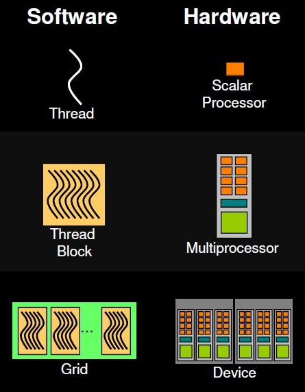
**Source of image: nvidia.com**
The term "device" is a general reference to the GPU, whereas the term "host" is reserved for the CPU. We often refer a scalar processor to a GPU "core".
So, when a GPU kernel is executed, each thread block is assigned to an SM. A maximum number of thread blocks can be assigned to an SM, depending on GPU hardware resources. The runtime system maintains a list of active blocks and assigns new blocks to SMs when resources are freed or in other words: once a thread block is assigned to an SM the resources on it are reserved until the execution of all threads in the block is not finished. Each thread block execution is independent from another (no synchronization can be done among blocks). Threads in each block are divided into warps of consecutive threads (generally 32 on modern GPU architectures) and the scheduler selects warps for execution from the residing blocks in an SM. A warp executes one common set of instructions at a time and a GPU "core" (scalar processor) executes one thread in the warp.
#### CUDA thread hierarchy
Let's recap everything in terms of the GPU CUDA thread hierarchy with some details:
- threads are organized into blocks: blocks can be 1D, 2D, 3D
- blocks are organized into a grid: grids can also be 1D, 2D, 3D
- each block or thread has a unique ID: `.x`, `.y`, `.z` are components in every dimension
- built-in variables for the CUDA thread hierarchy are:
- `threadIdx`: thread coordinate inside the block
- `blockIdx`: block coordinate inside the grid
- `blockDim`: block dimension in thread units
- `gridDim`: grid dimension in block units
The image below shows an example of a CUDA thread hierarchy with 2D blocks.
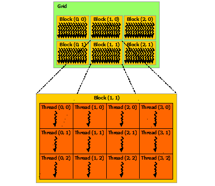
**Source of image: nvidia.com**
Using built-in variables we can define global thread indices that run in a kernel. For a 1D kernel we can define a global thread index `idx` in the following way:
~~~c
int idx = blockIdx.x * blockDim.x + threadIdx.x;
~~~
Similarly, we can define global thread indices `i` and `j` for a 2D kernel:
~~~c
int i = blockDim.x * blockIdx.x + threadIdx.x;
int j = blockDim.y * blockIdx.y + threadIdx.y;
~~~
Can you also define global thread indices for a 3D kernel?
These indices are defined as internal variables in a kernel and can be used for thread related computing. We have already seen such an index in the Hello World CUDA example where the index was defined to identify blocks only
~~~c
int idx = blockIdx.x;
~~~
and later used to print the block ID number
~~~c
printf("Hello world! I'm a thread in block %d\n", idx);
~~~
You could instead define a global thread index `gid`
~~~c
int gid = blockIdx.x * blockDim.x + threadIdx.x;
~~~
and print it with
~~~c
printf("Hello world! I'm a global thread index %d in hierarchy\n", gid);
~~~
Of course, the global thread index range is between 0 to `NUM_BLOCKS * BLOCK_SIZE - 1` if the `hello` kernel is invoked with:
~~~c
hello<<<NUM_BLOCKS, BLOCK_SIZE>>>();
~~~
One should remember that the kernel on the GPU is run with all the threads defined by the launch parameters in the triple chevron syntax `<<<...>>>` but the calculation could be limited, e.g., with an `if` clause:
~~~c
__global__ void hello(int N){
int gid = blockIdx.x * blockDim.x + threadIdx.x;
if(gid < N)
printf("Hello world! I'm a global thread index %d in hierarchy\n", gid);
}
~~~
For example, if one sets `N = 7` (note that `N` is an integer variable defined outside the kernel, hence it must be called as an input parameter in a function like manner), the kernel invoked by
~~~c
int N = 7;
hello<<<4, 2>>>(N);
~~~
would print global thread indices in the range from 0 to 6 instead of the total 0 to 7 deployed by invoking the kernel. You can experiment yourself by changing the launch parameters and value of `N`.
#### OpenCL work-item hierarchy
The GPU OpenCL work-item hierarchy is equivalent to the CUDA thread hierarchy except for terminology and some minor details:
- work-items are organized into work-groups
- the number of work-items can be specified in a work-group – this is called the local (work-group) size
- both work-items and work-groups can be 1D, 2D, 3D
- each work-item and work-group has a unique ID: `(0)`, `(1)`, `(2)` are components in every dimension
- built-in variables for the OpenCL work-item hierarchy are:
- `get_local_id`, equivalent to `threadIdx`
- `get_group_id`, equivalent to `blockIdx`
- `get_local_size`, equivalent to `blockDim`
- `get_global_id`, equivalent to `blockIdx * blockDim + threadIdx`
The image below shows an example of an OpenCL work-item hierarchy with 2D work-groups (note that the equivalent of "grid" in OpenCL is called NDRange).
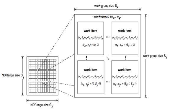
**Source of image: khronos.org**
Like CUDA, we can use built-in variables in OpenCL to define global work-item indices that run in a kernel. For a 1D kernel we can define a global work-item index `idx` in the following way:
~~~c
int idx = get_group_id(0) * get_local_size(0) + get_local_id(0);
~~~
This is unnecessary since OpenCL offers the `get_global_id` variable that returns a global work-item index:
~~~c
int idx = get_global_id(0);
~~~
Like in CUDA, we can define global work-item indices `i` and `j` for a 2D kernel in OpenCL with
~~~c
int i = get_group_id(0) * get_local_size(0) + get_local_id(0);
int j = get_group_id(1) * get_local_size(1) + get_local_id(1);
~~~
or equivalently with
~~~c
int i = get_global_id(0);
int j = get_global_id(1);
~~~
Can you once again define global work-item indices for a 3D kernel?
Like in CUDA, these indices are defined in a kernel as internal variables and can be used for work-item related computing in OpenCL. You can modify the Hello World OpenCL example to print the global work-item index and experiment with launch parameters along with an `if` clause in the kernel to limit the printout of indices.
See also:
[CUDA Programming Model](https://docs.nvidia.com/cuda/cuda-c-programming-guide/index.html#programming-model)
[OpenCL 1.2 API and C Language Specification ](https://www.khronos.org/registry/OpenCL/specs/opencl-1.2.pdf)
### 5.10 Vector addition on GPU
A standard introductory example for GPU computing is vector addition. We will first show how it is done on a CPU and then on a GPU. In the next two steps, we will use this example to present a step-by-step approach to GPU programming, both in CUDA and OpenCL.
Vector addition on a CPU can be done with a `for` loop. Each iteration computes the sum of one component of vectors `a` and `b`. The vector sum is stored in `out`.
~~~c
for(int i = 0; i < N; i++){
out[i] = a[i] + b[i];
}
~~~
You can have a look at the program for vector addition in C and execute it.
[](https://colab.research.google.com/drive/1vx1FVQ3xLgAAkndJD7mK5sebh1tjNsyj)
By now, we should know how to transform this `for` loop into a GPU kernel. The only difference is that the kernel in this case will take some extra parameters, i.e., the vectors `a`, `b`, `out` and the vector size `n`. Let's write down the CUDA kernel first:
~~~c
__global__ void vector_add(double *out, double *a, double *b, int n)
{
int i = blockIdx.x * blockDim.x + threadIdx.x;
if(i < n)
out[i] = a[i] + b[i];
}
~~~
You can see that the input parameters for the kernel `vector_add` are defined in a function like manner and that the index `i`, defined inside the kernel, represents the global thread index. In that way, the kernel sums the vector components in parallel (keep in mind that this is true if enough resources on the GPU are available): for every component addition, there's a thread that takes care of the computing task, while the `if` clause makes sure that the calculations are done only within the vector size. In the next step, we will see how the kernel is called, and how the parameters or variables must be defined.
For the same task, we can use an OpenCL kernel instead:
~~~c
__kernel void vector_add(__global double *a, __global double *b, __global double *out, int n) {
int i = get_global_id(0);
if(i < n)
out[i] = a[i] + b[i];
}
~~~
You can see that the kernel looks basically the same, except for variable type prefixes and built-in variables. In the next steps, we will also see how the kernel in OpenCL is called, and how the parameters or variables must be defined.
If you are curious about the codes for vector addition on GPU, you can have look at the CUDA version
[](https://colab.research.google.com/drive/18G29WIWRwaPgT_cg-rorHM1joPusiSml)
and the OpenCL version
[](https://colab.research.google.com/drive/1-EnE5A7haX3RWyaP2ebm5-sbIuPf4Ydd)
Don't be afraid if you find them difficult to grasp. We will explore and explain them step-by-step in the following steps.
### 5.11 CUDA step-by-step
In this step, we will look at vector addition in CUDA, which is a typical GPU program in CUDA, in detail. A typical CUDA program flow consists of the following steps:
- Allocate GPU memory
- Populate GPU memory with inputs from the host (CPU)
- Execute a GPU kernel on those inputs
- Transfer outputs from the GPU back to the host (CPU)
- Free GPU memory
We have to mention that recent NVIDIA GPUs (Pascal microarchitecture or newer) support unified memory (invoked with `cudaMallocManaged()`) in a single-pointer-to-data model. This means CPUs and GPUs can use the same memory address space. Consequently, transfers from/to GPU memory are no longer needed or are less important in a GPU accelerated code.
Let's analyze the *CUDA vector addition code* step-by-step and explain how to compile it into an executable program.
[](https://colab.research.google.com/drive/18G29WIWRwaPgT_cg-rorHM1joPusiSml)
**1\. Initialize device**
The first available CUDA device (GPU) is automatically set to `0`, but you can set it yourself by:
~~~c
CudaSetDevice(0);
~~~
Such initialization is important in multi GPU systems where there's a need for switching from one device to another, e.g., switching to device `1` can be done with:
~~~c
CudaSetDevice(1);
~~~
It's a good approach to initialize CUDA with:
~~~c
CUDA_ERROR(cudaSetDevice(0));
~~~
This call makes use of a custom defined error wrapper `CUDA_ERROR()`:
~~~c
/* CUDA error wraper */
static void CUDA_ERROR(cudaError_t err)
{
if (err != cudaSuccess) {
printf("CUDA ERROR: %s, exiting\n", cudaGetErrorString(err));
exit(-1);
}
}
~~~
This way, a CUDA program will continue with execution only if a CUDA capable device is available. Sometimes it is useful to get the device properties with `cudaGetDeviceProperties()`:
~~~c
cudaDeviceProp prop;
CUDA_ERROR(cudaGetDeviceProperties(&prop,0));
printf("Found GPU '%s' with %g GB of global memory, max %d threads per
block, and %d multiprocessors\n", prop.name,
prop.totalGlobalMem/(1024.0*1024.0*1024.0),
prop.maxThreadsPerBlock,prop.multiProcessorCount);
~~~
All the above calls are optional but it is a good approach to control CUDA initialization to avoid running GPU accelerated codes on unresponsive GPUs. Older CUDA versions also needed the inclusion of CUDA specific headers, e.g.
~~~c
#include <cuda.h>
#include <cuda_runtime.h>
#include <device_launch_parameters.h>
~~~
that are now redundant. Still, you can put these lines at the beginning of CUDA codes to no harm.
**2\. Allocate GPU memory**
Memory allocation on the device is done with `cudaMalloc()`:
~~~c
cudaMalloc((void**)&d_a, sizeof(double) * N);
cudaMalloc((void**)&d_b, sizeof(double) * N);
cudaMalloc((void**)&d_out, sizeof(double) * N);
~~~
For every variable on the host (CPU), from/to which GPU memory transfers will be done, we must allocate memory on the GPU of the same size and type.
It is also a good approach to use "d" for the variables in GPU memory as an indication for device, e.g., `d_a` or `a_d`. This naming convention is optional but quite useful in terms of code readability.
**3\. Transfer data from host to device memory**
Data transfer from host (CPU) to device (GPU) is done with `cudaMemcpy()` and the option `cudaMemcpyHostToDevice`. In the example of vector addition, we have to transfer data from host variables `a` and `b` to device variables `d_a` and `d_b`:
~~~c
cudaMemcpy(d_a, a, sizeof(double) * N, cudaMemcpyHostToDevice);
cudaMemcpy(d_b, b, sizeof(double) * N, cudaMemcpyHostToDevice);
~~~
We transfer the values of the components of vectors `a` and `b` from host do device memory. Note that host and device variables must be of the same size and type.
**4\. Execute kernel on device variables as inputs**
After transferring the components of vectors `a` and `b` from host do device memory, we can sum the vector components in parallel on the GPU. In the previous step, we have already shown how to do that, i.e., with the kernel `vector_add`:
~~~c
__global__ void vector_add(double *out, double *a, double *b, int n)
{
int i = blockIdx.x * blockDim.x + threadIdx.x;
if(i < n)
out[i] = a[i] + b[i];
}
~~~
Before executing the kernel, we have to define launch parameters, i.e., the number of threads per block and the number of blocks. We need at least 2020 threads in total. Choosing 1024 as the number of threads per block, we need 1.97 blocks (2020/1024) or rounded 2 blocks. We can do this calculation with
~~~c
int threadsPerBlock = 1024;
int blocksPerGrid = N/threadsPerBlock + (N % threadsPerBlock == 0 ? 0:1);
~~~
or alternatively with
~~~c
int threadsPerBlock = 1024;
int blocksPerGrid =(N + threadsPerBlock - 1) / threadsPerBlock;
~~~
Now we can launch the kernel with these parameters:
~~~c
vector_add<<<blocksPerGrid, threadsPerBlock>>>(d_out, d_a, d_b, N);
~~~
Note that we launched the kernel with the allocated device variables `d_out`, `d_a` and `d_b` as is usually done with function calls. Also, note that integers and constant type variables can be passed to the kernel without device memory allocation. In this case, we passed the vector size `N` in this way.
**5\. Transfer data back from device to host**
The kernel `vector_add` calculates the vector sum of `d_a` and `d_b` and puts it into the variable `d_out`. This variable, together with the vector sum, resides in GPU global memory and cannot be accessed by the CPU directly, hence it has to be transferred back to host memory to the variable `out`. This is done with `cudaMemcpy()` with a different option, `cudaMemcpyDeviceToHost`:
~~~c
cudaMemcpy(out, d_out, sizeof(double) * N, cudaMemcpyDeviceToHost);
~~~
Again, the counterpart host variable `out` must be of the same size and type as the device variable `d_out`.
**6\. Deallocate (free) device memory**
In the end (after the device variables are not needed anymore), we can free the allocated device memory:
~~~c
cudaFree(d_a);
cudaFree(d_b);
cudaFree(d_out);
~~~
**7\. Compiling the code**
CUDA codes reside in `*.cu` files, and the NVIDIA CUDA (nvcc) compiler can be used to compile them, e.g., in the case of the vector addition CUDA code:
~~~bash
!nvcc -o vector_add_cuda vector_add_cuda.cu
~~~
The executable can be run with:
~~~c
!./vector_add_cuda
~~~
Hardware design, number of cores, cache size, and supported arithmetic instructions are different for different GPU models. Every NVIDIA GPU supports a compute capability according to its microarchitecture, e.g., the Tesla V100 (Volta microarchitecture) supports CUDA compute capabilities up to 7.0 (see the output in **GPUs by numbers**). The above code can be compiled specifically for the V100 in the following way:
~~~bash
!nvcc -arch=sm_70 -gencode=arch=compute_70,code=sm_70 -o vector_add_cuda vector_add_cuda.cu
~~~
You can compile and run the CUDA vector addition code in the notebook. Check the output to see if the GPU calculates the vector sum correctly.
[CUDA Programming Guide](https://docs.nvidia.com/cuda/cuda-c-programming-guide/index.html)
### 5.12 OpenCL step-by-step
In this step, we will look at vector addition in OpenCL in detail. A typical OpenCL program flow basically consists of the same steps as a CUDA program flow, but you will notice that OpenCL is a more low-level programming extension with many calls to the OpenCL API. OpenCL, like CUDA, can also offer shared memory (Shared Virtual Memory) for host and device kernels, thus eliminating costly data transfers between host and device (supported only in OpenCL 2.0 and above). Unfortunately, the NVIDIA GPUs support only OpenCL 1.2 and the before-mentioned features are not available. For that reason, we will follow this standard to explain GPU accelerated programming in OpenCL.
Let's analyze the *OpenCL vector addition code* step-by-step and explain how to compile it into an executable program.
[](https://colab.research.google.com/drive/1-EnE5A7haX3RWyaP2ebm5-sbIuPf4Ydd)
**1\. Initialize device**
As opposed to CUDA, a specific OpenCL header must be included at the beginning of the code, depending on the operating system:
~~~c
#ifdef __APPLE__
#include <OpenCL/opencl.h>
#else
#include <CL/cl.h>
#endif
~~~
Before initializing the device, it's necessary to get platform and device information. This is more or less standard needed code that you can copy/paste to every OpenCL code. Device initialization consists of the following steps:
- declare context:
~~~c
cl_context context = clCreateContext(NULL, 1, &device_id, NULL, NULL, &ret);
~~~
- choose a device from context:
~~~c
ret = clGetDeviceIDs(platform_id, CL_DEVICE_TYPE_ALL, 1, &device_id, &ret_num_devices);
~~~
- create a command queue with device and context:
~~~c
cl_command_queue command_queue = clCreateCommandQueue(context, device_id, 0, &ret);
~~~
This code snippet is basically the same for every OpenCL program.
**2\. Create buffers and memory transfer to device**
Next, we create buffers which is essentially memory allocation on the GPU:
~~~c
cl_mem a_mem_obj = clCreateBuffer(context, CL_MEM_READ_ONLY, N * sizeof(double), NULL, &ret);
cl_mem b_mem_obj = clCreateBuffer(context, CL_MEM_READ_ONLY, N * sizeof(double), NULL, &ret);
cl_mem out_mem_obj = clCreateBuffer(context, CL_MEM_WRITE_ONLY, N * sizeof(double), NULL, &ret);
~~~
Notice, that we used the flag `CL_MEM_READ_ONLY` to create buffers for vectors `a` and `b` since the GPU kernel will only read the data. The vector sum will be stored in the buffer `out_mem_obj`, and the GPU kernel will only write to it, hence the use of the `CL_MEM_WRITE_ONLY` flag. If there's the need for both reading from and writing to memory buffers, one could use the flag `CL_MEM_READ_WRITE`.
After buffer creation, we can transfer host data to the device. Transfering the host variables `a` and `b` to GPU memory buffers `a_mem_obj` and `b_mem_obj` is done with the following calls:
~~~c
ret = clEnqueueWriteBuffer(command_queue, a_mem_obj, CL_TRUE, 0, N * sizeof(double), a, 0, NULL, NULL);
ret = clEnqueueWriteBuffer(command_queue, b_mem_obj, CL_TRUE, 0, N * sizeof(double), b, 0, NULL, NULL);
~~~
Like in CUDA, the size and the type of the memory buffers of the device variables must be the same as for the host counterparts, in this case: `N * sizeof(double)`.
**3\. Build program and select kernel**
You have probably noticed that the kernel source was loaded at the beginning with:
~~~c
FILE *fp;
char *source_str;
size_t source_size;
fp = fopen("vector_add.cl", "r");
if (!fp) {
fprintf(stderr, "Failed to load kernel.\n");
exit(1);
}
source_str = (char*)malloc(MAX_SOURCE_SIZE);
source_size = fread( source_str, 1, MAX_SOURCE_SIZE, fp);
fclose( fp );
~~~
These lines basically load the OpenCL kernel `vector_add` for vector addition (shown in **Vector addition on GPU**)
~~~c
__kernel void vector_add(__global double *a, __global double *b, __global double *out, int n) {
int i = get_global_id(0);
if(i < n)
out[i] = a[i] + b[i];
}
~~~
as a string from the file `vector_add.cl`. It's common practice in OpenCL programming to have kernels in `*.cl` files, but one could also define them in the main code as plain strings.
With the kernel source loaded, we can create a program from it
~~~c
cl_program program = clCreateProgramWithSource(context, 1, (const char **)&source_str, (const size_t *)&source_size, &ret);
~~~
build the program
~~~c
ret = clBuildProgram(program, 1, &device_id, NULL, NULL, NULL);
~~~
and create the OpenCL kernel
~~~c
cl_kernel kernel = clCreateKernel(program, "vector_add", &ret);
~~~
Notice the constant use of the variable `ret` of the `cl_int` type defined at the beginning. This variable accepts return values for the OpenCL API. As said before, you can use many of the OpenCL API calls as boiler-plate code as long as you are consistent with the variable definitions in these calls.
**4\. Set arguments and enqueue kernel**
After the creation of the OpenCL kernel, we have to first set its arguments with:
~~~c
ret = clSetKernelArg(kernel, 0, sizeof(cl_mem), (void *)&a_mem_obj);
ret = clSetKernelArg(kernel, 1, sizeof(cl_mem), (void *)&b_mem_obj);
ret = clSetKernelArg(kernel, 2, sizeof(cl_mem), (void *)&out_mem_obj);
ret = clSetKernelArg(kernel, 3, sizeof(cl_int), (void *)&n);
~~~
These arguments must follow the same order (indices from 0 to 3) as in the kernel definition:
~~~c
vector_add(__global double *a, __global double *b, __global double *out, int n)
~~~
Notice that integer variables, e.g., `n` in this case, do not need the creation of a memory buffer but still need to be set as a kernel argument.
Next, we must set local and global work-group sizes:
~~~c
size_t local_item_size = 1024;
int n_blocks = n/local_item_size + (n % local_item_size == 0 ? 0:1);
size_t global_item_size = n_blocks * local_item_size;
~~~
This is equivalent to setting the number of threads per block and the number of blocks per grid in CUDA.
Finally, we execute the kernel with:
~~~c
ret = clEnqueueNDRangeKernel(command_queue, kernel, 1, NULL, &global_item_size, &local_item_size, 0, NULL, NULL);
~~~
You will notice that the execution of a kernel in OpenCL is different than in CUDA. The main difference is that the kernel in OpenCL is not called in a function-like manner, i.e., with passing arguments to it. In OpenCL, the arguments of a kernel are set with the `clSetKernelArg()` API function before the kernel is executed. On the other hand, launch parameters for the kernel, i.e., `global_item_size` and `local_item_size` are set at kernel execution, like in CUDA.
**5\. Transfer back results**
The kernel `vector_add` calculates the vector sum of `a_mem_obj` and `b_mem_obj` and puts it into the memory buffer `out_mem_obj`. Like in CUDA, this vector sum resides in GPU global memory and cannot be accessed by the CPU directly, hence it has to be transferred back to host memory to the variable `out`. The transfer is done with:
~~~c
ret = clEnqueueReadBuffer(command_queue, out_mem_obj, CL_TRUE, 0, N * sizeof(double), out, 0, NULL, NULL);
~~~
**6\. Free buffers and resources**
In the end, we can free the memory buffers
~~~c
ret = clReleaseMemObject(a_mem_obj);
ret = clReleaseMemObject(b_mem_obj);
ret = clReleaseMemObject(out_mem_obj);
~~~
as well as other resources
~~~c
ret = clFlush(command_queue);
ret = clFinish(command_queue);
ret = clReleaseKernel(kernel);
ret = clReleaseProgram(program);
ret = clReleaseCommandQueue(command_queue);
ret = clReleaseContext(context);
~~~
**7\. Compiling the code**
OpenCL codes reside in `*.c` files (main code) and `*.cl` files (kernels). Compilers that can link to the OpenCL library (generally with the flag `-lOpenCL`) can be used, e.g., `gcc` or `nvcc`. One should be aware that for running OpenCL codes on a GPU, a Software Developer Kit (SDK) must be installed. For NVIDIA GPUs, the installation of the CUDA SDK is enough and compiling can be done with:
~~~bash
!nvcc -o vector_add_opencl vector_add_opencl.c -lOpenCL
~~~
For non-NVIDIA GPUs or CPUs one could compile the code with, e.g.:
~~~bash
!gcc -o vector_add_opencl vector_add_opencl.c -lOpenCL
~~~
Of course, OpenCL drivers for the hardware must be installed, generally, as implementations for OpenCL called Installable Client Drivers (ICDs).
As before, you can compile and run the OpenCL vector addition code in the notebook. Check the output to see if the GPU calculates the vector sum correctly.
[OpenCL 1.2 Reference Pages](https://www.khronos.org/registry/OpenCL/sdk/1.2/docs/man/xhtml/)
[OpenCL 1.2 API and C Language Specification ](https://www.khronos.org/registry/OpenCL/specs/opencl-1.2.pdf)
[OpenCL 1.2 Extensions Specification](https://www.khronos.org/registry/OpenCL/specs/opencl-1.2-extensions.pdf)
[OpenCL 1.2 Quick Reference Card](https://www.khronos.org/registry/OpenCL/sdk/1.2/docs/OpenCL-1.2-refcard.pdf)
### 5.13 CUDA and OpenCL comparison
To sum up, we will give a side by side comparison of both the GPU programming models discussed so far. We haven't looked at everything that you will find in the comparison tables. Some things we will discuss later in the upcoming steps, for others you can have a look at the documentation for CUDA and OpenCL.
#### Execution model terminology
| CUDA | OpenCL |
| :---------------------------: | :---------------: |
| SM (Streaming Multiprocessor) | CU (Compute Unit) |
| thread | work-item |
| block | work-group |
| global memory | global memory |
| constant memory | constant memory |
| shared memory | local memory |
| local memory | private memory |
#### Function, variable and built-in variable types
| CUDA | OpenCL |
| :-----------------------------: | :---------------: |
| `__global__ function` | `__kernel function` |
| `__device__ function` | `function` |
| `__constant__ variable` | `__constant variable` |
| `__device__ variable` | `__global variable` |
| `__shared__ variable` | `__local variable` |
| `gridDim` | `get_num_groups()` |
| `blockDim` | `get_local_size()` |
| `blockIdx` | `get_group_id()` |
| `threadIdx` | `get_local_id()` |
| `blockIdx * blockDim + threadIdx` | `get_global_id()` |
| `gridDim * blockDim` | `get_global_size()` |
#### Kernel synchronization
| CUDA | OpenCL |
| :------------------: | :---------------: |
| `__syncthreads()` | `barrier()` |
| `__threadfence()` | / |
| `__threadfence_block()` | `mem_fence()` |
| / | `read_mem_fence()` |
| / | `write_mem_fence()` |
#### API calls
| CUDA | OpenCL |
| :-----------------------: | :---------------: |
| `cudaGetDeviceProperties()` | `clGetDeviceInfo()` |
| `cudaMalloc()` | `clCreateBuffer()` |
| `cudaMemcpy()` | `clEnqueueReadBuffer()`, `clEnqueueWriteBuffer()` |
| `cudaFree()` | `clReleaseMemObj()` |
| `kernel<<<...>>>()` | `clEnqueueNDRangeKernel()` |
### 5.14 CUDA and OpenCL programming and execution models
This quiz tests your knowledge about the basics of CUDA and OpenCL programming and execution models.
1. What statements about CUDA and OpenCL are correct? (multiple choice answer):
[ ] both CUDA and OpenCL supported by many GPU vendors
[x] CUDA is supported only by NVIDIA GPUs, while OpenCL by many GPU vendors
[x] CUDA and OpenCL execution models are similar, but with a different terminology
[ ] CUDA and OpenCL execution models are different
Correct.
2. Which of the following correctly describes the relationship between warps, thread blocks and CUDA cores?
( ) a warp is divided into one or more thread blocks and each thread block executes on a single CUDA core
( ) a thread block is divided into one or more warps and each warp executes on a single CUDA core
(x) a thread block is divided into one or more warps and in each warp, every thread executes on a separate CUDA core
Correct. Each CUDA core executes a different thread from a single warp.
3. In a CPU, what is the closest equivalent of a GPU warp?
( ) float
(x) vector
( ) thread
( ) core
4. A function with the `__global__` or `__kernel` prefix can be called from the host or the device and can run on either of them.
( ) true
(x) false
Correct. This prefix specifies that the function can be called from either host or device, but it runs on the device alone.
5. Which of the following correctly describes a GPU kernel?
( ) a kernel may contain a mix of host and GPU code
(x) all thread blocks (work-groups with work-items) involved in the same computation use the same kernel
( ) a kernel is part of the GPU's internal micro-operating system, allowing it to act as in independent host
Correct.
6. Threads in a thread block (work-items in a work-group) can be distributed across two or more streaming multiprocessors (SMs).
( ) true
(x) false
Correct. A thread block (work-group) must be run entirely on a single SM.
7. Which internal variable in OpenCL is used to identify the work-item among all other work-items executed in the kernel?
( ) `get_local_id()`
(x) `get_global_id()`
( ) `blockIdx`
( ) `threadIdx`
Correct.
8. CPUs and GPUs can use the same memory address space:
( ) for every CUDA and OpenCL version on every GPU architecture
(x) for newer CUDA and OpenCL versions and newer GPU architectures
( ) for CUDA versions only
( ) same memory address space is not supported yet
Correct.
9. Threads in CUDA or work-items in OpenCL can synchronize in:
(x) in a single block (work-group)
( ) in many blocks (work-groups) associated with a single kernel
( ) can not synchronize
Correct. Threads (work-items) can synchronize only in shared (local) memory in a single block (work-group).
10. Which of the following statements is true with regard to compute capability in CUDA?
( ) code compiled for hardware of one compute capability will not need to be re-compiled to run on hardware of another
(x) different compute capabilities may imply a different amount of local memory per thread
( ) compute capability is measured by the number of FLOPS a GPU accelerator can compute
Correct. Every NVIDIA GPU supports a compute capability according to its microarchitecture and associated hardware design, number of cores, cache size and supported arithmetic instructions.
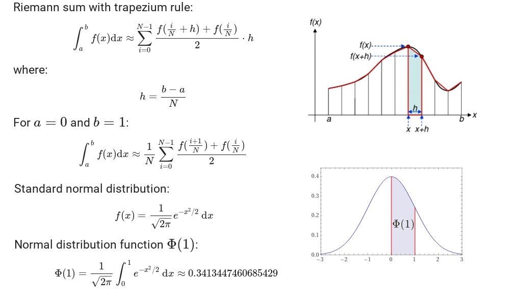
### 5.15 Numerical integration: Riemann sum with trapeziums
We are ready for a more complex example in numerical computation to show some extra features of GPU computing: Riemann sum for numerical integration. First, let's show how it's done on a CPU, and after that think of how can we parallelize it on the GPU with CUDA and OpenCL. We will also parallelize the CPU version with OpenMP to show how to also off-load the computation on GPU with OpenMP.
A definite integral of a function can be approximated using the trapezium rule. The area under the function on the interval from a to b, which represents the definite integral, is divided into N trapeziums. The area of each trapezium is equal to the median of the trapezium `(f(x+h)+f(x))/2` multiplied with the sub-interval width `(b-a)/N`. The sum of all trapezium areas is an approximation of the definite integral of the function from a to b. For simplicity, we choose `a = 0` and `b = 1` to calculate the normal distribution function from 0 to 1, which is equal to 0.3413447460685429 (see picture below).
How can we do this example on the CPU? The simplest approach is to use a `for` loop to calculate trapezium medians and trapezium sums:
~~~c
double riemann(int n)
{
double sum = 0;
for(int i = 0; i < n; ++i)
{
double x = (double) i / (double) n;
double fx = (exp(-x * x / 2.0) + exp(-(x + 1 / (double)n) * (x + 1 / (double)n) / 2.0)) / 2.0;
sum += fx;
}
sum *= (1.0 / sqrt(2.0 * M_PI)) / (double) n;
return sum;
}
~~~
In the code above, we calculate trapezium medians for every sub-interval and add them to the `sum` variable at every iteration. In the end, we multiply this sum of trapezium medians with `(1.0 / sqrt(2.0 * M_PI)) / (double) n` to obtain the Riemann sum. The term `1.0 / (double) n` is in fact the height of the trapezium `(b-a)/n` and is the same for every trapezium since the sub-interval width is the same and we have chosen `a = 0` and `b = 1`.
The whole Riemann sum CPU code can be found in the following notebook.
[](https://colab.research.google.com/drive/1LBqOcLlPN1zAczCh5uaA1C2Xa_gLoy0x)
If you compile the code for `N` equal to 1 billion, i.e.
~~~c
#define N 1000000000
~~~
without optimization the calculation of the Riemann sum will take about 90 seconds. With the `-O3` optimization level flag the calculation with the compiled code will take less than half of the time, about 40 seconds.
But can we do better, e.g., with some parallelization approach like OpenMP? We shall see the answer in the next step.
See also:
[Riemann Sum](https://mathworld.wolfram.com/RiemannSum.html)
[Trapezoidal (Trapezium) Rule](https://mathworld.wolfram.com/TrapezoidalRule.html)
[Normal Distribution Function](https://mathworld.wolfram.com/NormalDistributionFunction.html)
### 5.16 Riemann sum with OpenMP
In Week 2 of this course, you have learned how to use OpenMP to parallelize parts of the code and speed up the execution. In this exercise, you will use this knowledge and try to speed up the calculation of the Riemann sum code from the previous step.
Complete the following tasks:
- use OpenMP to parallelize the `for` loop in the Riemann sum C code from the previous step
- execute the code for the maximum threads available on the CPU (hint: use `!lscpu` to get information on the CPU)
Did you succeed to gain any speed up with the use of OpenMP? Leave a comment with your findings.
If you have any troubles modifying the code or compiling it, you can have a look at the solution given in the notebook below.
[](https://colab.research.google.com/drive/1x1kDCOkkZZ60v5AI5Qh_woB6M8dahP1l)
### 5.17 OpenMP off-loading to GPU for Riemann sum
OpenMP is an example of a directive-based method that can be used to off-load computation-intensive tasks to GPUs. From OpenMP 4.0 on, new device constructs have been added to support this. As in CUDA or OpenCL, the execution model relies on the host on which the OpenMP program begins execution and then off-loads tasks or data to a target device, e.g., GPU.
The main OpenMP device constructs are:
- `target`
- `teams`
By defining a `target` construct, a new target task is generated. When the latter starts, the enclosed target region is executed by an initial thread running sequentially on a target device if it's available and supported. If not, all target regions associated with the device are executed on the host. The `teams` construct generates a league of thread teams where the master thread of each team executes the region sequentially, as shown on the image below.
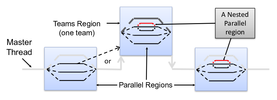
**Source of image: OpenMP Accelerator Model, IWOMP 2016**
Some important OpenMP 4.x device constructs are listed in the following table:
| Device construct | Description |
| ------------------------- | -------------------------------------------------------------------------------- |
| `#pragma omp target` | Map variables to a device data environment and execute the construct on the device. |
| `#pragma omp target data` | Creates a data environment for the extent of the region. |
| `#pragma omp declare target` | A declarative directive that specifies that variables and functions are mapped to a device. |
| `#pragma omp teams` | Creates a league of thread teams where the master thread of each team executes the region. |
| `#pragma omp distribute` | Specifies loops which are executed by the thread teams. |
| `#pragma omp ... simd` | Specifies code that is executed concurrently using SIMD instructions. |
| `#pragma omp distribute parallel for` | Specifies a loop that can be executed in parallel by multiple threads that are members of multiple teams. |
So, how can we off-load the computation of the Riemann sum to the GPU using OpenMP? We start from the OpenMP directive in the previous exercise. If you have completed it successfully, then you should have come to a solution something like:
~~~c
double riemann(int n)
{
double sum = 0;
#pragma omp parallel for reduction(+:sum)
for(int i = 0; i < n; ++i)
{
double x = (double) i / (double) n;
sum += (exp(-x * x / 2.0) + exp(-(x + 1 / (double)n) * (x + 1 / (double)n) / 2.0)) / 2.0;
}
sum *= (1.0 / sqrt(2.0 * M_PI)) / (double) n;
return sum;
}
~~~
To the OpenMP directive:
~~~c
#pragma omp parallel for reduction(+:sum)
~~~
we just have to add appropriate device constructs to enable off-loading to a GPU, i.e.:
~~~c
#pragma omp target teams distribute parallel for simd map(tofrom: sum) map(to: n) reduction(+:sum)
~~~
Here `map` is used to copy data from the host to the device and vice versa, e.g., `map(tofrom: sum)` copies the variable `sum` to the device (GPU) and after computation back to the host (CPU), while `map(to: n)` just copies the variable `n` to the device.
The complete function for calculating the Riemann sum with OpenMP GPU off-loading is as follows:
~~~c
double riemann(int n)
{
double sum = 0;
#pragma omp target teams distribute parallel for simd map(tofrom: sum) map(to: n) reduction(+:sum)
for(int i = 0; i < n; ++i)
{
double x = (double) i / (double) n;
sum += (exp(-x * x / 2.0) + exp(-(x + 1 / (double)n) * (x + 1 / (double)n) / 2.0)) / 2.0;
}
sum *= (1.0 / sqrt(2.0 * M_PI)) / (double) n;
return sum;
}
~~~
Such OpenMP off-loading to the GPU results in speed up greater than in typically many threads OpenMP execution on the host. It is quite close to classical GPU acceleration with CUDA or OpenCL, provided the device (GPU) is supported, and compilers can build programs with OpenMP off-load.
You can have a look at the whole code in the following notebook.
[](https://colab.research.google.com/drive/1Zbum3NETtjJvwzFfOIk3puaf_yMvNWjU)
You can see that the code is compiled with the `-fopenmp` flag as with normal OpenMP codes, but two other flags are added: `-foffload=-lm` for using a specific math library on the GPU and `-fno-stack-protector` to disable buffer overflow checks. The latter flag has to be added on Ubuntu systems, while the former is needed with the GCC compiler. Note that for GCC on Ubuntu a special offloading compiler to NVPTX, e.g., `gcc-8-offload-nvptx` and a plugin for offloading to NVPTX `libgomp-plugin-nvptx1` must be installed. On other systems and with other compilers, e.g., with CLANG/LLVM, other flags are used when compiling OpenMP off-loading to GPU codes. One should also keep in mind that GPU libraries, e.g., CUDA for NVIDIA cards, must be installed for successful off-loading to GPUs with OpenMP or OpenACC.
[IWOMP 2016 Tutorial: OpenMP Accelerator Model](https://iwomp2016.riken.jp/wp-content/uploads/2016/10/tutorial-accelerator.pdf)
[Webinar: Intro to GPU Programming with the OpenMP API](https://www.openmp.org/events/intro-to-gpu-programming-with-the-openmp-api/)
[Offloading Support in GCC](https://gcc.gnu.org/wiki/Offloading)
### 5.18 Riemann sum with one GPU kernel
When off-loading codes or part of codes to GPUs, the easiest approach is to search for parts that are embarrassingly parallel, which can be directly (with minimum changes) ported to a GPU programming extension.
In the case of the Riemann sum,
~~~c
for(int i = 0; i < n; ++i)
{
double x = (double) i / (double) n;
double fx = (exp(-x * x / 2.0) + exp(-(x + 1 / (double)n) * (x + 1 / (double)n) / 2.0)) / 2.0;
sum += fx;
}
~~~
an embarrassingly parallel part is the calculation of trapezium medians `fx` since it is independent. On the other hand, adding the calculated trapezium median to the `sum` at every iteration is a typical sequential task not suited for GPU parallelization. It naturally follows that the calculation of trapezium medians should be off-loaded to the GPU while adding them should be done sequentially on the host (CPU).
#### CUDA kernel `medianTrapezium`
A suitable CUDA kernel for the calculation of trapezium medians should be something like this:
~~~c
__global__ void medianTrapezium(double *a, int n)
{
int idx = blockIdx.x * blockDim.x + threadIdx.x;
double x = (double)idx / (double)n;
if(idx < n)
a[idx] = (exp(-x * x / 2.0) + exp(-(x + 1 / (double)n) * (x + 1 / (double)n) / 2.0)) / 2.0;
}
~~~
Here `a` is an array of calculated trapezium medians that has to be returned to the host. The kernel is almost identical to the `for` loop with the global thread index `idx` taking the role of `i`.
Adding the medians is done simply with a for loop on the host, as well as the calculation of the Riemann sum:
~~~c
double sum = 0;
for (int i=0; i < n; i++) sum += a_h[i];
sum *= (1.0 / sqrt(2.0 * M_PI)) / (double)n;
~~~
The array `a_h` is the host counter-part of the device array `a_d`. They are both initialized and allocated at the beginning with:
~~~c
double* a_h = (double *)malloc(size);
double* a_d; cudaMalloc((double **) &a_d, size);
~~~
The kernel is executed with:
~~~c
int block_size = 1024;
int n_blocks = n/block_size + (n % block_size == 0 ? 0:1);
medianTrapezium <<< n_blocks, block_size >>> (a_d, n);
~~~
Only the transfer from device to host is needed since the array of trapezium medians is calculated on the device (GPU):
~~~c
cudaMemcpy(a_h, a_d, sizeof(double)*n, cudaMemcpyDeviceToHost);
~~~
#### OpenCL kernel `medianTrapezium`
An equivalent OpenCL kernel is of the form:
~~~c
__kernel void medianTrapezium(__global double *a, int n) {
int idx = get_global_id(0);
double x = (double)idx / (double)n;
if(idx < n)
a[idx] = (exp(-x * x / 2.0) + exp(-(x + 1 / (double)n) * (x + 1 / (double)n) / 2.0)) / 2.0;
}
~~~
Again, adding the medians is done again with a for loop on the host, as well as the calculation of the Riemann sum. The array `a` is the host counter-part of the memory buffer `a_mem_obj`, i.e., the array on the device. Both are allocated at the beginning with:
~~~c
double *a = (double*)malloc(sizeof(double)*n);
cl_mem a_mem_obj = clCreateBuffer(context, CL_MEM_READ_WRITE, n * sizeof(double), NULL, &ret);
~~~
The kernel is initialized and executed with:
~~~c
cl_kernel kernel = clCreateKernel(program, "medianTrapezium", &ret);
ret = clSetKernelArg(kernel, 0, sizeof(cl_mem), (void *)&a_mem_obj);
ret = clSetKernelArg(kernel, 1, sizeof(cl_int), (void *)&n);
size_t local_item_size = 1024;
int n_blocks = n/local_item_size + (n % local_item_size == 0 ? 0:1);
size_t global_item_size = n_blocks * local_item_size;
ret = clEnqueueNDRangeKernel(command_queue, kernel, 1, NULL, &global_item_size, &local_item_size, 0, NULL, NULL);
~~~
Again, only the transfer from device to host is needed, since the array of trapezium medians is calculated on the device (GPU):
~~~c
ret = clEnqueueReadBuffer(command_queue, a_mem_obj, CL_TRUE, 0, n * sizeof(double), a, 0, NULL, NULL);
~~~
### 5.19 Profiling of the Riemann sum codes with one GPU kernel
In this exercise, you will execute the CUDA and OpenCL Riemann sum codes with one GPU kernel and compare their performance to CPU and OpenMP codes. You will also do a profiling of the codes to identify possible bottlenecks.
Execute the CUDA Riemann sum code
[](https://colab.research.google.com/drive/17XdBdkOWpiToW-Hcdb8MjMdtf7FHnBNR)
and the OpenCL Riemann sum code
[](https://colab.research.google.com/drive/1dvgXHfyap5Ql47BKIl2kCcewYVyFRnPy)
with `N` equal to 1 billion. Compare the execution time of the codes. Which is faster? What's the speed up compared to CPU and OpenMP codes?
Use `nvprof` to profile the execution of the CUDA code. Can you identify the bottleneck?
Analyze the diagnostic outputs of the OpenCL code. Can you identify the bottleneck for this code also? Note that execution time measurements of the GPU parts by the CPU are not necessarily trustful.
### 5.20 Sum reduction
In the exercise of the previous step, you have profiled the GPU Riemann sum codes with one kernel. The profiling gave you information on the bottlenecks of the code: memory transfer from device (GPU) to host (CPU) of the array of trapezium medians and the calculation in a `for` loop of the sum of medians.
The profiling results of the first version (with one kernel) of the GPU Riemann sum codes give you the idea of what should be avoided in GPU programming: time-consuming memory transfers from host (CPU) to device (GPU) and vice versa. The transfer of the array of trapezium medians to the host took 5 seconds, more than half of the total execution time of the code! This is hardly a surprise since an array of 1 billion double-precision float elements occupies more than 8 GB in host or device memory. It should be noted that the manipulation of such big arrays is not a good approach in GPU programming: first, the GPU global memory is limited, and second, access to this memory even by the GPU itself is quite slow. We used such a big array only for demonstration purposes.
But how can we get rid of the bottlenecks of memory transfer and sum calculation on the host? A hint to a solution was already given in the OpenMP codes: sum reduction. While parallel reductions in OpenMP are quite easily achieved, this is not the case in CUDA or OpenCL since they have to be done programmatically. One approach or a variant of sum reduction is shown in the image below.
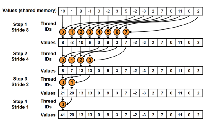
**Source of image: nvidia.com**
Let’s assume we have an array of 16 elements in shared memory. How can we add these elements in terms of sum reduction?
- Step 1: We add the values with IDs 0 and 8 and store the sum into ID 0 of the next array. Likewise, we do the same for IDs 1–7 and 9–15. Stride = 8 means that we add elements strided by 8 positions. The results are stored in the next array with IDs 0–7. So, we actually reduced the previous array of 16 elements into an array of 8 elements.
- Step 2: We reduce the stride by half (Stride = 4), meaning we add the values with IDs 0 and 4 and store the sum into ID 0 of the next array. Likewise, we do the same for IDs 1–3 and 5–7. The results are stored in the next array with IDs 0–3. Again, we reduced the previous array by half: from 8 to 4 elements.
- Step 3: We again reduce the stride by half (Stride = 2), meaning we add the values with IDs 0 and 2 and store the sum into ID 0 of the next array. Likewise, we do the same for IDs 1 and 3. The results are stored in the next array with IDs 0–1. By that, we reduced the previous array from 4 to 2 elements.
- Step 4: In the last iteration, we have Stride = 1 since we have just 2 elements in the array. We just add the values of these elements with IDs 0 and 1 to get the final sum.
This kind of parallel reduction is called sequential addressing. If we have an array of N elements, we can do a parallel reduction in log<sub>2</sub>N steps. Programmatically we can do this kind of reduction with a reversed loop and strided threadID-based indexing. We will show in the next step how this is done in CUDA and OpenCL. We must also explain why reduction should be done with striding in shared memory. As you probably noticed in the comparison tables, the GPUs have different types of memories. Global memory is the slowest, and therefore access to it should be reduced to a minimum. Instead, shared memory (CUDA) or local memory (OpenCL) should be used. This type of memory is much faster than global memory but can be used only in a block of threads (or work-group of work-items). In it, threads or work-items can be synchronized. Striding access to memory is used to achieve coalescing, i.e., combining multiple memory accesses into a single transaction.
[Optimizing Parallel Reduction in CUDA](https://developer.download.nvidia.com/assets/cuda/files/reduction.pdf)
### 5.21 Riemann sum with parallel reduction on GPU
Let's show how to perform a parallel sum reduction described in the previous step with a GPU kernel. The sum reduction kernel will be added to the previous GPU codes, both in CUDA and OpenCL, to get rid of the bottlenecks.
#### Parallel reduction in CUDA
Sequential addressing with a reversed loop and strided threadID-based indexing described in the previous step can be done in CUDA in the following way:
~~~c
for (int size = block_size/2; size>0; size/=2) {
if (idx<size)
r[idx] += r[idx+size];
__syncthreads();
}
~~~
The variable `block_size` is the initial size of the array on which sum reduction is performed. On every next iteration, striding is reduced by half (`size/=2`). Every thread `idx` adds up two elements in the array strided by the current `size` to an element `r[idx]` of the array `r` in shared memory. For synchronization of threads in the block, `__syncthreads()` is used.
Because the block size on the GPU is limited (maximum number of threads per block) to 1024 (see GPUs by numbers), we can use an array of maximum 1024 elements to perform parallel reduction. If we have to sum up an array of more than 1024 elements, we must use more than one block or reduce the array in global memory to an array in shared memory. The latter can be done, e.g., by:
~~~c
int idx = threadIdx.x;
double sum = 0;
for (int i = idx; i < n; i += block_size)
sum += a[i];
extern __shared__ double r[];
r[idx] = sum;
__syncthreads();
~~~
Here the array `a` of trapezium medians of size `n` in global memory is reduced to the array `r` of size `block_size` in shared memory. Using more blocks in shared memory would be, of course, a better approach in terms of performance, but for simplicity, we will use just one block of threads. Ultimately, the sum of trapezium medians in the sum reduction kernel is obtained by:
~~~c
if (idx == 0)
*out = r[0];
~~~
The whole code of the `reducerSum` kernel in CUDA is as follows:
~~~c
__global__ void reducerSum(double *a, double *out, int n, int block_size) {
int idx = threadIdx.x;
double sum = 0;
for (int i = idx; i < n; i += block_size)
sum += a[i];
extern __shared__ double r[];
r[idx] = sum;
__syncthreads();
for (int size = block_size/2; size>0; size/=2) {
if (idx<size)
r[idx] += r[idx+size];
__syncthreads();
}
if (idx == 0)
*out = r[0];
}
~~~
This kernel is executed after the kernel `medianTrapezium`, which calculates the array of trapezium medians `a`. This array is available in the GPU global memory for the kernel `reducerSum` for sum reduction of the trapezium medians. It is executed in the following way:
~~~c
int block_size = 1024;
int n_blocks2 = 1;
reducerSum <<< n_blocks2, block_size, block_size*sizeof(double) >>> (a_d, out, n, block_size);
~~~
As explained, we use 1 block with 1024 threads for sum reduction. You will notice an additional parameter in the triple chevron syntax: `block_size*sizeof(double)`. This parameter is needed for the array `r` in shared memory, which is primarily allocated on the host with:
~~~c
double* r = (double *)malloc(block_size * sizeof(double));
~~~
#### Parallel reduction in OpenCL
Sequential addressing with a reversed loop and strided work-item ID-based indexing can be done in OpenCL in the following way:
~~~c
for (int size = block_size/2; size>0; size/=2) {
if (idx<size)
r[idx] += r[idx+size];
barrier(CLK_LOCAL_MEM_FENCE);
}
~~~
The `for` loop is identical as in CUDA, except for work-items synchronization in the work-group achieved with `barrier(CLK_LOCAL_MEM_FENCE)`.
Similarly, the reduction of the array in global memory to an array in shared memory is achieved with:
~~~c
int idx = get_local_id(0);
double sum = 0;
for (int i = idx; i < n; i += block_size)
sum += a[i];
r[idx] = sum;
barrier(CLK_LOCAL_MEM_FENCE);
~~~
The sum of trapezium medians in the sum reduction kernel is obtained as before by:
~~~c
if (idx == 0)
*out = r[0];
~~~
The whole code of the `reducerSum` kernel in OpenCL is as follows:
~~~c
__kernel void reducerSum(__global double *a, __global double *out, __local double *r, int n, int block_size)
{
int idx = get_local_id(0);
double sum = 0;
for (int i = idx; i < n; i += block_size)
sum += a[i];
r[idx] = sum;
barrier(CLK_LOCAL_MEM_FENCE);
for (int size = block_size/2; size>0; size/=2) {
if (idx<size)
r[idx] += r[idx+size];
barrier(CLK_LOCAL_MEM_FENCE);
}
if (idx == 0)
*out = r[0];
}
~~~
Notice that the OpenCL kernel uses an additional parameter `__local double *r` for the array in local memory (the equivalent of shared memory in CUDA). We could have done the same for the CUDA kernel instead of defining `r` as an internal kernel variable in shared memory. Like in CUDA, this kernel is executed after the kernel `medianTrapezium` and is executed in the following way:
~~~c
int block_size = 1024;
cl_kernel kernel2 = clCreateKernel(program, "reducerSum", &ret);
ret = clSetKernelArg(kernel2, 0, sizeof(cl_mem), (void *)&a_mem_obj);
ret = clSetKernelArg(kernel2, 1, sizeof(cl_mem), (void *)&out_mem_obj);
ret = clSetKernelArg(kernel2, 2, block_size * sizeof(cl_double), NULL);
ret = clSetKernelArg(kernel2, 3, sizeof(cl_int), (void *)&n);
ret = clSetKernelArg(kernel2, 4, sizeof(cl_int), (void *)&block_size);
size_t local_item_size2 = block_size;
size_t global_item_size2 = block_size;
ret = clEnqueueNDRangeKernel(command_queue, kernel2, 1, NULL, &global_item_size2, &local_item_size2, 0, NULL, NULL);
~~~
As before, we use 1 block (work-group) with 1024 threads (work-items) for sum reduction since the global item size is equal to the local item size of 1024.
### 5.22 Profiling of the Riemann sum codes with two GPU kernels
In this exercise you will execute the CUDA and OpenCL Riemann sum codes with two GPU kernels and compare their performance to CPU, OpenMP codes and codes with one GPU kernel. You will also do profiling of the codes to see if we have gotten rid of the bottlenecks.
Execute the CUDA Riemann sum code with two kernels
[](https://colab.research.google.com/drive/199tA6Df9xMbI7YgdIu0IPpnuA1CV-Nhi)
and the OpenCL Riemann sum code with two kernels
[](https://colab.research.google.com/drive/1TXsCj_veelAtp4DC8JEhYOpYsZWKE_jF)
with `N` equal to 1 billion. Compare the execution time of the codes. Which is faster? What's the speed up compared to CPU, OpenMP codes and codes with one GPU kernel?
Use `nvprof` to profile the execution of the CUDA code. How much time does the kernel `reducerSum` take to execute? Have the bottlenecks been solved?
Analyze the diagnostic outputs of the OpenCL code. Have the bottlenecks gotten solved, too? Keep in mind that execution time measurements of the GPU parts by the CPU are not necessarily trustworthy.
### 5.23 Visual profiling and tracing of the GPU codes
In this step, we will present some tools for visual profiling and tracing of the GPU codes. These tools are generally available with the GPU SDK, some of them can also be installed separately. The tools can't be invoked through Jupyter notebooks directly, but you can try them if you have access to a system with direct command-line or GUI execution. Profiling and tracing are useful in terms of code performance analysis and hints at optimization.
Tools capable of profiling and/or tracing CUDA and OpenCL codes:
CUDA:
- **nvprof**: command line profiling tool from CUDA toolkit (deprecated in CUDA 11)
- **nvvp**: visual profiler (GUI) tool from CUDA toolkit (deprecated in CUDA 11)
- [**Nvidia Nsight Systems**](https://developer.nvidia.com/nsight-systems)
- [**TAU** (Tuning and Analysis Utilities)](http://www.cs.uoregon.edu/research/tau/home.php): open source tool for profiling and tracing
- other tools: [**Vampir**](https://vampir.eu/), [**Scalasca**](https://www.scalasca.org/) (for large scale applications)...
OpenCL:
- on NVIDIA cards: **OpenCL profiling not supported since CUDA 8**
- on AMD cards: OpenCL profiling with [**Radeon GPU profiler**](https://gpuopen.com/rgp/)
- **TAU** (Tuning and Analysis Utilities): open source tool for profiling and tracing
- other tools: **Vampir**, [**Intel VTune Profiler**](https://www.intel.com/content/www/us/en/developer/tools/oneapi/vtune-profiler.html#gs.mgnxel)...
### Profiling and tracing of CUDA codes
You already know how to use the profiling tool `nvprof`, e.g., for the CUDA Riemann sum code with two kernels
```
$ nvprof ./riemann_cuda_double_reduce
```
you obtained the following output in command line (see the previous step Profiling of the Riemann sum codes with two GPU kernels):
```
==2194== NVPROF is profiling process 2194, command: ./riemann_cuda_double_reduce
Found GPU 'Tesla K80' with 11.173 GB of global memory, max 1024 threads per block, and 13 multiprocessors
CUDA kernel 'medianTrapezium' launch with 976563 blocks of 1024 threads
CUDA kernel 'reducerSum' launch with 1 blocks of 1024 threads
Riemann sum CUDA (double precision) for N = 1000000000 : 0.34134474606854243
Total time (measured by CPU) : 2.130000 s
==2194== Profiling application: ./riemann_cuda_double_reduce
==2194== Profiling result:
Type Time(%) Time Calls Avg Min Max Name
GPU activities: 79.45% 668.84ms 1 668.84ms 668.84ms 668.84ms reducerSum(double*, double*, int, int)
20.55% 172.96ms 1 172.96ms 172.96ms 172.96ms medianTrapezium(double*, int)
0.00% 8.4480us 1 8.4480us 8.4480us 8.4480us [CUDA memcpy DtoH]
API calls: 46.26% 1.01224s 3 337.41ms 10.109us 1.00527s cudaFree
38.47% 841.87ms 1 841.87ms 841.87ms 841.87ms cudaMemcpy
14.56% 318.66ms 2 159.33ms 587.33us 318.07ms cudaMalloc
0.34% 7.3509ms 582 12.630us 305ns 476.82us cuDeviceGetAttribute
0.27% 6.0104ms 6 1.0017ms 998.14us 1.0108ms cuDeviceTotalMem
0.05% 1.1714ms 1 1.1714ms 1.1714ms 1.1714ms cudaGetDeviceProperties
0.03% 589.12us 6 98.187us 95.529us 103.46us cuDeviceGetName
0.01% 267.51us 2 133.76us 23.377us 244.14us cudaLaunchKernel
0.00% 31.279us 6 5.2130us 2.8280us 15.291us cuDeviceGetPCIBusId
0.00% 10.163us 1 10.163us 10.163us 10.163us cudaSetDevice
0.00% 6.6350us 12 552ns 392ns 1.2660us cuDeviceGet
0.00% 3.6970us 3 1.2320us 417ns 2.0400us cuDeviceGetCount
0.00% 2.4670us 6 411ns 357ns 584ns cuDeviceGetUuid
```
Tracing can be done with `nvvp`, e.g., for the CUDA Riemann sum code with two kernels:
```
$ nvvp ./riemann_cuda_double_reduce
```
Visual profiling can be invoked with many options for analysis of the CUDA code. The picture below shows the traces for the Riemann sum code with two kernels and the summary of both kernels execution (average duration, FLOP, multiprocessor occupancy...).
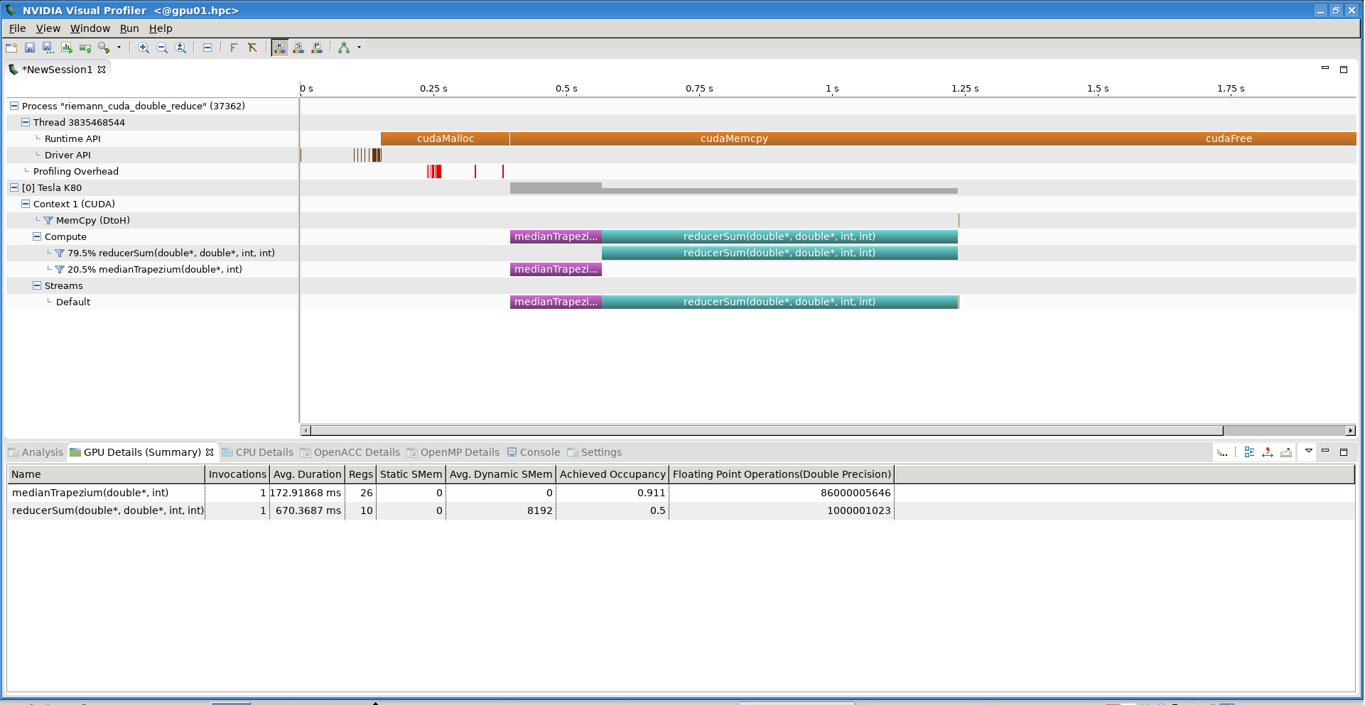
One can observe from the traces that the kernel `reducerSum` is executed after the kernel `medianTrapezium` and that for the latter 91.1% Streaming Multiprocessor (SM) occupancy was achieved with 86000005646 Double Precision Floating Point Operations (Flop) in 172.91868 milliseconds. For the kernels, the parameters can be shown graphically, e.g., the performance in Flops. You can calculate the latter yourself from data in the summary, e.g., for the kernel `medianTrapezium`:
86000005646/172.91868*1000/10^9 = 497.34 GFlops
You can then compare this performance to the theoretical FP64 (double) performance of 1371 GFlops for the Tesla K80 GPU (on which the CUDA program was executed) and determine the efficacy of the code.
As already pointed out, the tools `nvprof` and `nvvp` are already deprecated in CUDA 11 and will be discontinued. They are replaced by Nvidia Nsight Systems. The equivalent of `nvprof` in the command line is `nsys`. One can profile the CUDA Riemann sum code with two kernels in the following way:
```
$ nsys profile --trace cuda ./riemann_cuda_double_reduce
$ nsys stats report1.qdrep
```
First, we generate the profiling report `report1.qdrep` of which the output can be subsequently invoked in the command line by the `nsys stats` call:
```
Time(%) Total Time (ns) Num Calls Average Minimum Maximum Name
------- --------------- --------- ------------- ----------- ----------- ----------------
79.7 614,696,365 1 614,696,365.0 614,696,365 614,696,365 cudaMemcpy
19.5 150,392,555 2 75,196,277.5 170,492 150,222,063 cudaMalloc
0.8 5,854,639 3 1,951,546.3 2,800 5,766,738 cudaFree
0.0 41,361 2 20,680.5 7,670 33,691 cudaLaunchKernel
Time(%) Total Time (ns) Instances Average Minimum Maximum Name
------- --------------- --------- ------------- ----------- ----------- --------------------------------------
96.7 594,399,821 1 594,399,821.0 594,399,821 594,399,821 reducerSum(double*, double*, int, int)
3.3 20,265,788 1 20,265,788.0 20,265,788 20,265,788 medianTrapezium(double*, int)
Time(%) Total Time (ns) Operations Average Minimum Maximum Operation
------- --------------- ---------- ------- ------- ------- ------------------
100.0 3,040 1 3,040.0 3,040 3,040 [CUDA memcpy DtoH]
```
The equivalent of `nvvp` is `nsys-ui`. By typing in the command line
```
$ nsys-ui
```
the Nsight Systems GUI will be invoked. One can then load the previously generated report `report1.qdrep` to visualize traces. The picture below shows the traces for the Riemann sum code with two kernels visualized by the Nsight Systems GUI.
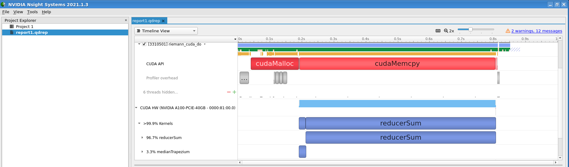
### Profiling and tracing of OpenCL codes
For profiling and tracing OpenCL codes, one can use the TAU Performance System. Unfortunately, it is not a part of GPU SDKs, therefore it must be installed separately.
Profiling of the OpenCL Riemann sum code with two kernels can be done with TAU in the following way. First, we generate profiles with:
```
$ tau_exec -T serial -opencl ./riemann_opencl_double_reduce
```
This will generate 2 profile files: `profile.0.0.0` and `profile.0.0.1`.
Profiling in command line can be done with:
```
$ pprof
```
The output is a detailed profiling report, we will show just an excerpt from it:
```
NODE 0;CONTEXT 0;THREAD 1:
---------------------------------------------------------------------------------------
%Time Exclusive Inclusive #Call #Subrs Inclusive Name
msec total msec usec/call
---------------------------------------------------------------------------------------
100.0 0.0165 767 1 3 767448 .TAU application
75.3 577 577 1 0 577820 reducerSum
24.7 189 189 1 0 189608 medianTrapezium
0.0 0.00275 0.00275 1 0 3 ReadBuffer
FUNCTION SUMMARY (total):
---------------------------------------------------------------------------------------
%Time Exclusive Inclusive #Call #Subrs Inclusive Name
msec total msec usec/call
---------------------------------------------------------------------------------------
100.0 20 2,035 2 34 1017668 .TAU application
37.6 766 766 1 0 766036 cl_int clEnqueueReadBuffer(cl_command_queue, cl_mem, cl_bool, size_t, size_t, void *, cl_uint, const cl_event *, cl_event *) C
28.4 577 577 1 0 577820 reducerSum
12.7 258 258 1 0 258078 cl_int clBuildProgram(cl_program, cl_uint, const cl_device_id *, const char *, void (*)(cl_program, void *), void *) C
9.3 189 189 1 0 189608 medianTrapezium
7.9 160 160 1 0 160755 cl_context clCreateContext(const cl_context_properties *, cl_uint, const cl_device_id *, void (*)(const char *, const void *, size_t, void *), void *, cl_int *) C
2.0 41 41 1 0 41175 cl_int clGetPlatformIDs(cl_uint, cl_platform_id *, cl_uint *) C
1.0 21 21 2 0 10596 cl_int clEnqueueNDRangeKernel(cl_command_queue, cl_kernel, cl_uint, const size_t *, const size_t *, const size_t *, cl_uint, const cl_event *, cl_event *) C
0.0 0.279 0.279 1 0 279 cl_int clReleaseProgram(cl_program) C
0.0 0.025 0.025 2 0 12 cl_kernel clCreateKernel(cl_program, const char *, cl_int *) C
0.0 0.024 0.024 1 0 24 cl_command_queue clCreateCommandQueue(cl_context, cl_device_id, cl_command_queue_properties, cl_int *) C
0.0 0.011 0.011 2 0 6 cl_int clReleaseKernel(cl_kernel) C
0.0 0.011 0.011 2 0 6 cl_mem clCreateBuffer(cl_context, cl_mem_flags, size_t, void *, cl_int *) C
0.0 0.01 0.01 1 0 10 cl_int clFlush(cl_command_queue) C
0.0 0.009 0.009 1 0 9 cl_program clCreateProgramWithSource(cl_context, cl_uint, const char **, const size_t *, cl_int *) C
0.0 0.006 0.006 1 0 6 cl_int clReleaseCommandQueue(cl_command_queue) C
0.0 0.006 0.006 7 0 1 cl_int clSetKernelArg(cl_kernel, cl_uint, size_t, const void *) C
0.0 0.004 0.004 1 0 4 cl_int clFinish(cl_command_queue) C
0.0 0.004 0.004 2 0 2 cl_int clGetKernelInfo(cl_kernel, cl_kernel_info, size_t, void *, size_t *) C
0.0 0.003 0.003 1 0 3 cl_int clReleaseContext(cl_context) C
0.0 0.00275 0.00275 1 0 3 ReadBuffer
0.0 0.002 0.002 1 0 2 cl_int clGetDeviceIDs(cl_platform_id, cl_device_type, cl_uint, cl_device_id *, cl_uint *) C
0.0 0.001 0.001 2 0 0 cl_int clGetCommandQueueInfo(cl_command_queue, cl_command_queue_info, size_t, void *, size_t *) C
```
The GUI profiling utility can be invoked with:
```
$ paraprof
```
The visualisation of profiles (threads), i.e., one profile for OpenCL API calls and the other for OpenCL kernels, can be seen on the pictures below.
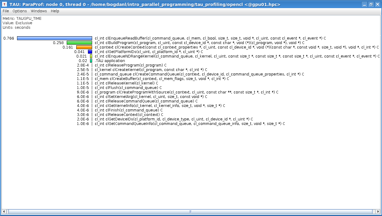
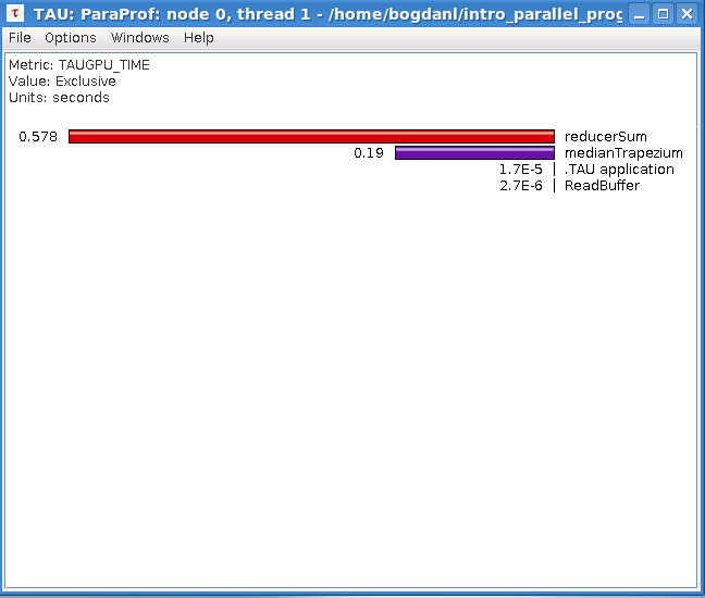
Tracing of the OpenCL Riemann sum code with two kernels can be done with TAU in the following way. Again, we first generate traces (`tautrace.0.0.0.trc` and `tautrace.0.0.1.trc`) with:
```
$ TAU_TRACE=1 tau_exec -T serial -opencl ./riemann_opencl_double_reduce
```
Then we can use the `jumpshot` utility within TAU to visualize the traces:
```
$ tau_treemerge.pl
$ tau2slog2 tau.trc tau.edf -o tau.slog2
$ jumpshot tau.slog2
```
On the pictures below you can see the traces with the description legend.
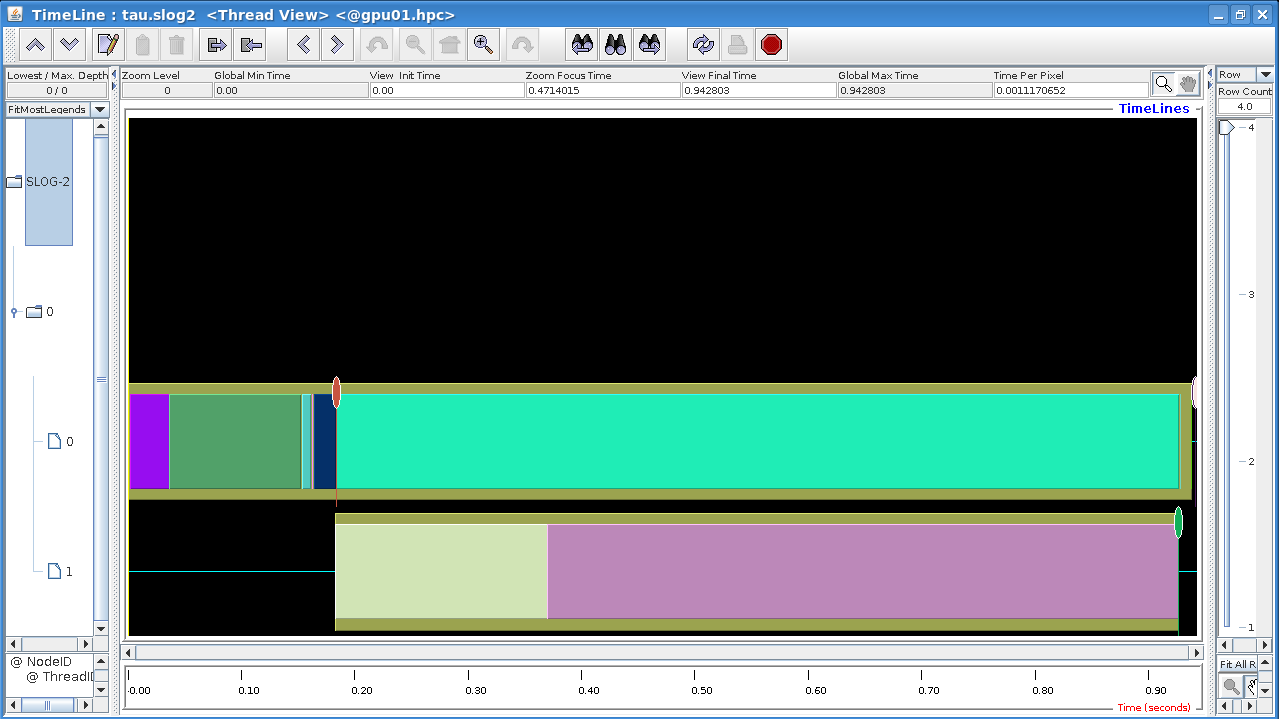
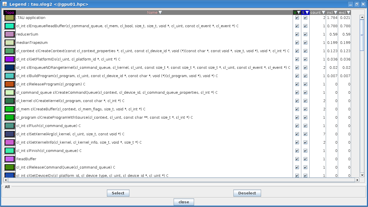
The second trace (thread 1) shows the OpenCL kernels on a timeline: it is evident that the `reducerSum` kernel is executed after the `medianTrapezium` kernel, as is the case of the trace showing CUDA kernels.
The latter observation should be clarified in some detail. In CUDA all operations executed on the device belong to the so-called default stream. Multiple kernels submitted to the same stream are executed consequently one after another. If one needs concurrent execution of multiple kernels, then every kernel must be defined in a different stream. For synchronization of kernels execution, one can use `cudaDeviceSynchronize()`, which is in fact a blocking call, i.e., it blocks any further execution until the device (GPU) has finished all the tasks launched to that point.
Similarly, multiple OpenCL kernels enqueued in the same command queue are executed consequently one after another. Concurrent execution of multiple kernels is achieved by creating multiple command queues.
### 5.24 Test on GPU parallelisation
With this test we will check your knowledge about using GPU for parallel programming.
Test available on FutureLearn in the MOOC [Introduction to Parallel Programming](https://www.futurelearn.com/courses/interactive-hands-on-introduction-to-parallel-programming).
### 5.25 Week 5 wrap-up
In this week we gave an introduction to Graphical Processing Units (GPUs) as a means to accelerate computing and introduced you to GPU architectures and GPU execution models. Step-by-step examples to the most widely used GPU programming extensions (CUDA and OpenCL), a brief introduction to OpenMP as a means to off-load computation to GPUs and a GPU numerical example should have prepared you to use accelerated programming approaches in your own codes.
We are interested in your opinion on the Week 5 content:
- did you find the introduction to the topic of GPU parallel computing easy to follow?
- did the examples in Jupyter notebooks work as expected?
- what were the parts of Week 5 that were the most difficult to understand?
- do you think GPU computation techniques you learned about will be useful for you?
### 5.26 Extra content: GPU programming in Python
In the introductory week you have also run the CUDA "Hello World!" example in Python, i.e., in PyCUDA. Both Python wrappers of CUDA and OpenCL exist, although not officially suported. As an extra content we give here Riemann sum scripts (with one kernel) in PyCUDA and PyOpenCL.
The scripts are available in the following notebook.
[](https://colab.research.google.com/drive/1bBC9O2qLTGbaQ0uSwpv0QRCfrmhx-nbi)
Compare the Python scripts with the appropriate equivalents in C and then run them. How close is their performance to that of the executable C programs?
Notice, that for running the scripts prior installation of the following libraries is needed, i.e., for PyCUDA:
~~~bash
!pip -q install pycuda
~~~
and for PyOpenCL:
~~~bash
!pip -q install pyopencl
~~~
See also:
[PyCUDA’s documentation](https://documen.tician.de/pycuda/)
[PyOpenCL’s documentation](https://documen.tician.de/pyopencl/)
###### tags: GPU