# A personalizable performance predictive model for mixed-terrain long distance cycling rides.
**Danilo Lessa Bernardineli**

## Abstract
*We introduce in this article a performance predictive model (PPM) that can be used and calibrated by amateur athletes for inferring moving time on long-distance & mixed-terrain bicycles routes, such as randonneuring and ultracycling events. We show that those can be utilized for a myriad of use cases, such as 1) ex-ante performance predictions under a variety of tactical & environmental scenarios, 2) classifying and planning segments across routes, 3) ex-post analysis of performance determinants, 4) ex-post analysis of counterfactuals. We proceed them to describe those applications through a series of case studies that was based on the usage of this model.*

## Introduction

- Why have a PPM?
- Uses of a PPM.
- Literature on PPMs
- Challenges on PPM for long-distance / mixed-terrain rides
- Problem Statement

### Literature Review

Olds et al. (1995, [2]) did present "a complete set of equations for a “first principles” mathematical model of road-cycling performance, including corrections for the effect of winds, tire pressure and wheel radius, altitude, relative humidity, rotational kinetic energy, drafting, and changed drag." while collecting field data that was then compared to the model predictions, which did result on a correlation of 0.89 (p>=0.1%). The model did use energetic demand and supply concepts and physiological sub-models for predicting (TODO)

Bertucci et al. (2013, [3]) did a field test in order to evaluate the aerodynamics and rolling resistance of mountain biking cyclists across 1) smooth vs knobby tyres; 2) lower pressure (29 Psi) vs higher pressure (58 Psi); 3) road vs grass vs sand terrain types. His finds includes that the effective frontal area ($Cd \cdot A$) of mountain bikers can be estimated to be around $0.357±0.023 m^2$ and that the mean aerodynamic resistance is typically on the order of $8\%-35\%$ of the total resistance to motion. The smooth tyre had $21\%±15\%$ less resistance than the knobby tyre, with the effect being most pronounced on road terrain but insignificant on non-road terrain. The mean resistive contribution of the rolling resistance across terrains was found to be $61\%±7\%$ on the grass, $35\%±5\%$ on the sand and $21\%±7\%$ on the road. By discussing and comparing to Grappe et al. (1999, [8]), the authors suggests that the rolling resistance in mountain biking can be expected to be roughly 2 to 3 times higher than on traditional road cycling.

Goff et al. (2012, [4]) did build a PPM for the winning times on the 2011 Tour de France stages on which the sum over all predicted stage times did miss the sum over all actual times by 0.5%. His model was based on an inclined-plane approach, where a single route was decomposed into a series of inclined-plane segments that were provided by the race organization. Assumptions were made for parameters such as rolling resistance ($C_{rr}=0.003$) and aerodynamics ($C_d A = 0.35 \text{ if uphill, } 0.25 \text{ if downhill}$). Power was estimated by using subjective choices based on angle cutoffs as described in Hannas et al. (2004, [9]).

Novak et al. (2018, [5]) did use a hierarchical multi linear regression model for predicting times on a 30-km cross-country mountain biking circuit with a 2% mean prediction accuracy. His model independent variables was composed of laboratory-derived measurements related to physiological, cognitive and technical individual functions, and one of his conclusions is that performance prediction on XCO-MTB events does requires a multi-dimensional approach. Novak et al. (2018, [7]) did reproduce that same approach, but for 4h mountain biking rides, with similar conclusions. It is pointed out that the heterogeneity between circuits in terms of steepness and terrain types has limited the applications of the previous performance prediction models to any use beyond the circuit used by the studies.

From this review, it is concluded that there's a gap on the literature on describing a PPM that can be readily applied to athletes to both long-distance and mixed-terrain cycling rides, such as randonneuring or ultracycling events. In particular, we lack a PPM that satisfies the key properties of 1) Can be calibrated by using field measurements by athletes; 2) Can be individually customized in terms of power profile strategy; 3) Can be generalized to predict over arbitrary mixed-terrain routes; This generates the rationale for the PPM that we'll introduce in the next section of this article.

---

[2]: Olds, T. S., Norton, K. I., Lowe, E. L., Olive, S., Reay, F., & Ly, S. (1995). Modeling road-cycling performance. Journal of applied physiology, 78(4), 1596-1611.

[3]: Bertucci, W. M., Rogier, S., & Reiser, R. F. (2013). Evaluation of aerodynamic and rolling resistances in mountain-bike field conditions. Journal of sports sciences, 31(14), 1606-1613.

[4]: Goff, J. E. (2012). Predicting winning times for stages of the 2011 Tour de France using an inclined-plane model. Procedia Engineering, 34, 670-675.

[5]: Andrew R. Novak, Kyle J. M. Bennett, Job Fransen & Ben J. Dascombe (2018) A multidimensional approach to performance prediction in Olympic distance cross-country mountain bikers, Journal of Sports Sciences, 36:1, 71-78, DOI: 10.1080/02640414.2017.1280611

[6]: Ben Piggott, Sean Müller, Paola Chivers, Carmen Papaluca & Gerard Hoyne (2019) Is sports science answering the call for interdisciplinary research? A systematic review, European Journal of Sport Science, 19:3, 267-286, DOI: 10.1080/17461391.2018.1508506

[7]: Andrew R. Novak, Kyle J. M. Bennett, Job Fransen & Ben J. Dascombe (2018) Predictors of performance in a 4-h mountain-bike race, Journal of Sports Sciences, 36:4, 462-468, DOI: 10.1080/02640414.2017.1313999

[8]: F. Grappe , R. Candau , B. Barbier , M. D. Hoffman , A. Belli & J.-D. Rouillon (1999) Influence of tyre pressure and vertical load on coefficient of rolling resistance and simulated cycling performance, Ergonomics, 42:10, 1361-1371, DOI: 10.1080/001401399185009

[9]: Hannas, B. L., & Goff, J. E. (2005). Inclined-plane model of the 2004 Tour de France. European Journal of Physics, 26(2), 251–259. doi:10.1088/0143-0807/26/2/004

\subsection{Inclined Plane Models}

## Model Overview

### Goals

To have a performance model on which 1) the free variables can be estimated solely with segment aggregated strategy, route and weather data; 2) allows for expression over differing counterfactuals with ease; 3) allows for performance determinants analysis.

### Energy Based Model

$$
\begin{align}
E_{\text{in}}&=E_{\text{out}} \\
\\
E_{\text{in}}&=E_l+E_w+E_{g-} \\
E_l &:= \text{Assumed or Measured} \\
E_w &:= \text{Assumed or Estimated} \\
E_{g-} &= mgh_-\\
\\
E_{\text{out}}&=E_a + E_r+E_{g+}+E_b+E_d \\
E_a &= C_d A \rho \int_0^t (v-w)^2 dt\\
E_r &= m g \int_0^dC_{rr}dx = mgd\langle C_{rr} \rangle \\
E_{g+} &= m g h_+ \\
E_b &= \int_0^tB(t)dt
\end{align}$$

---

$$E_l=E_a + E_r + E_{g+} + E_d + E_b - E_{g-} - E_w$$
$$E_\text{g-, eff} := E_{g-} - (E_a - E_\text{a, flat}) - E_b$$
$$E_\text{g-, eff} := \epsilon E_{g-}$$
$$E_l=E_\text{a, flat} + E_r + E_{g+} + E_d - \epsilon E_\text{$g-$} - E_w$$
$$v_\text{cf, flat} := \text{Computed by solving for $v_{gs}$ for a fixed power as a % of the average power}$$
$$E_\text{a, flat} = C_d A(v_\text{cf, flat}-w)^2$$
$$T=\frac{E_l}{\langle P \rangle}$$

---
$$\epsilon=1-\frac{E_\text{a, flat} - E_a -E_b}{E_{g-}}$$
$$\epsilon=1-\frac{E_\text{a, flat} - (E_l + E_{g-} + E_w - E_r - E_{g+} - E_d)}{E_{g-}}$$

---

$$T=\frac{d (mgC_{rr} + \frac{C_dA}{2}\rho(v-w)^2) + h_+ mg - h_- \epsilon mg}{P}$$

$$T =\frac{d+ h_+ mg \alpha - h_-\epsilon mg \alpha}{P \alpha}$$

The terms $E_a$ is unknown and needs to be estimated. The procedure that we take is as follows:
1. Compute the counterfactual flat speed given by $v_\text{cf, flat}$
2. Compute the counterfactual flat duration
3. Compute the counterfactual drag energy

As for the terms

#### Pure Climb

### Effective Distance Model

\begin{align}
T&=\frac{d}{v}= \frac{\tilde{d}}{\tilde{v}}\\
\tilde{d}&=d_f+\alpha h_+ + \beta h_-\\
\tilde{v}&=v_f\\
\end{align}

---

\begin{align}
\alpha &= \alpha_g (1-\epsilon) \\
\alpha_g &= \frac{v_f}{v_c} \\
v_c &= \frac{P_u}{mg} \\
\langle P_u \rangle &= (1-f_{c, t}) k_u \langle P \rangle + f_{c, t} \bar{P}
\end{align}

---

\begin{align}
v_f&=S+T-\frac{b}{3a} \\
S&=\sqrt[3]{R+\sqrt[3]{Q^3 + R^2}} \\
T&=\sqrt[3]{R-\sqrt[3]{Q^3 + R^2}} \\
Q&=\frac{3ac-b^2}{9a^2} \\
R&=\frac{9abc-27a^2d-2b^3}{5a^3}\\
a&= C_d A \rho\\
b&=v_w C_d A \rho\\
c&=m g (\sin{\theta} + C_{rr} \cos{\theta}) + \frac{C_d A \rho v_w^2}{2}\\
d&=-(1-\epsilon_c) \langle P \rangle\\
\end{align}

$$\theta = 0$$

---

\begin{align}
C_{rr} \approx f_{\text{paved}} C_{rr, \text{paved}} + (1 - f_{\text{paved}}) C_{rr, \text{unpaved}}
\end{align}

---

Parameter | Meaning | Unit | Affecting Factors
| - | - | - | -
$d$ | Distance | km | Route
$h_+$ | Cumulative uphill height | km | Route
$h_-$ | Cumulative downhill height | km | Route
$\epsilon$ | Rolling Terrain Coefficient | Unitless | Route, Local conditions, setup and tactics
$v_w$ | Headwind speed | - | Local conditions
$C_d A$ | Aerodynamic Drag | - | Local conditions, setup and tactics
$\beta$ | Downhill efficiency | - | Route, Local conditions, setup and tactics
$f_{\text{paved}}$ | Segment paved fraction | - | Route
$C_{rr, \text{paved}}$ | Paved Rolling Resistance | - | Route and tactics
$C_{rr, \text{unpaved}}$ | Unpaved Rolling Resistance | - | Route, local conditions and tactics
$m$ | Total mass | - | Setup
$k_u$ | Climbing Power Gain Factor | - | Tactics
$f_{c, t}$ | Fraction of Climbing Time at Threshold | - | Tactics
$\bar{P}$ | Threshold Power | - | Individual
$\epsilon_c$ | Mechanical efficiency | - | Setup
$\rho$ | Air Pressure | - | Route and local conditions
$g$ | Gravity | - | Route

Metric | Unit | Dimension
| - | - | -
$T$ | - | -
$\hat{d}$ | - | -

---

### Simplified Model

The effective distance $\hat{D}$ is given by:

$$\hat{D} = x + \alpha u + \beta d$$

While the estimated duration $\hat{t}$ is given by:
$$\hat{t} = \frac{\hat{D}}{\hat{v_f}}$$

$\alpha$ and $\beta$ are unitless parameters to be found, while $\hat{v_f}$ is an estimate of the average speed when adopting a specific power strategy (non-corrected by the wind)

A priori, the model parameters can be found statistically by doing linear regression on a dataset of existing rides that show similar profile, however, there are some rules of thumb which has show a good enough result when comparing empirically.

#### Finding $v_f$

This parameter is associated with the mean speed on a flat profile. A good enough estimate is to use interactive calculators for computing the expected speed at 70% FTP (ref 1). CdA can be estimated by using frontal area photos with a relatively good accuracy (ref 2).

Testing multiple values of CdA, weights and power outputs can generate a range of possible flat speeds that can be used for providing uncertainty.

#### Finding $\alpha$

This is associated with the theoretical maximum VAM and some effiency measure in regards to using stateful energy for overcoming short climbs.

$$\alpha = \alpha_g (1 - \epsilon_g)$$

$$\alpha_g = \frac{k_g}{\gamma}$$

$$k_g = \frac{P}{mg}$$

#### Wind Influence

$$\hat{v_f}^* \approx \hat{v_f} - \gamma u$$

#### Modified Power Strategy

Given the sensitivity of the estimated duration on the flat speed estimate and the non-linear dependences of marginal power into speed, one good estimate for the new speed $\hat{v_f}^*$ is given by:

$$\hat{v_f}^* = \hat{v_f} \sqrt{\frac{P_{new}}{P_{old}}}$$.

Supposing $P_{new} > P_{old}$, this correction tends to sub-estimate the estimate when the average speed is as slow such so that the dominating terms are the ones associated with linear dependencies (namely, rolling resistance and gravity). The opposite conclusion is made when the average speed is as fast such that the terms associated with aerodynamic drag dominates, although the scale of the error is less.

## Model Applications

### Ex-ante ride durations under varying assumptions

### Ex-post determinants for the ride durations

### Ex-post counterfactuals

## Case Studies

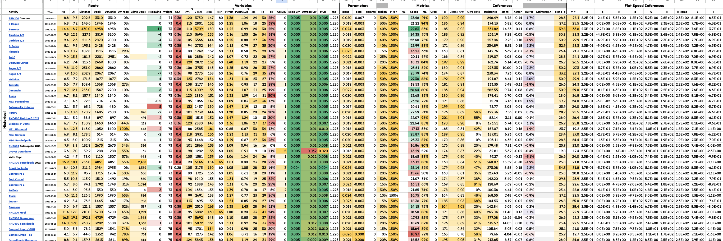
### Estimating Individual Parameters by fitting multiple activities

*Fig: Table containing predicted moving and elapsed times across many activities*

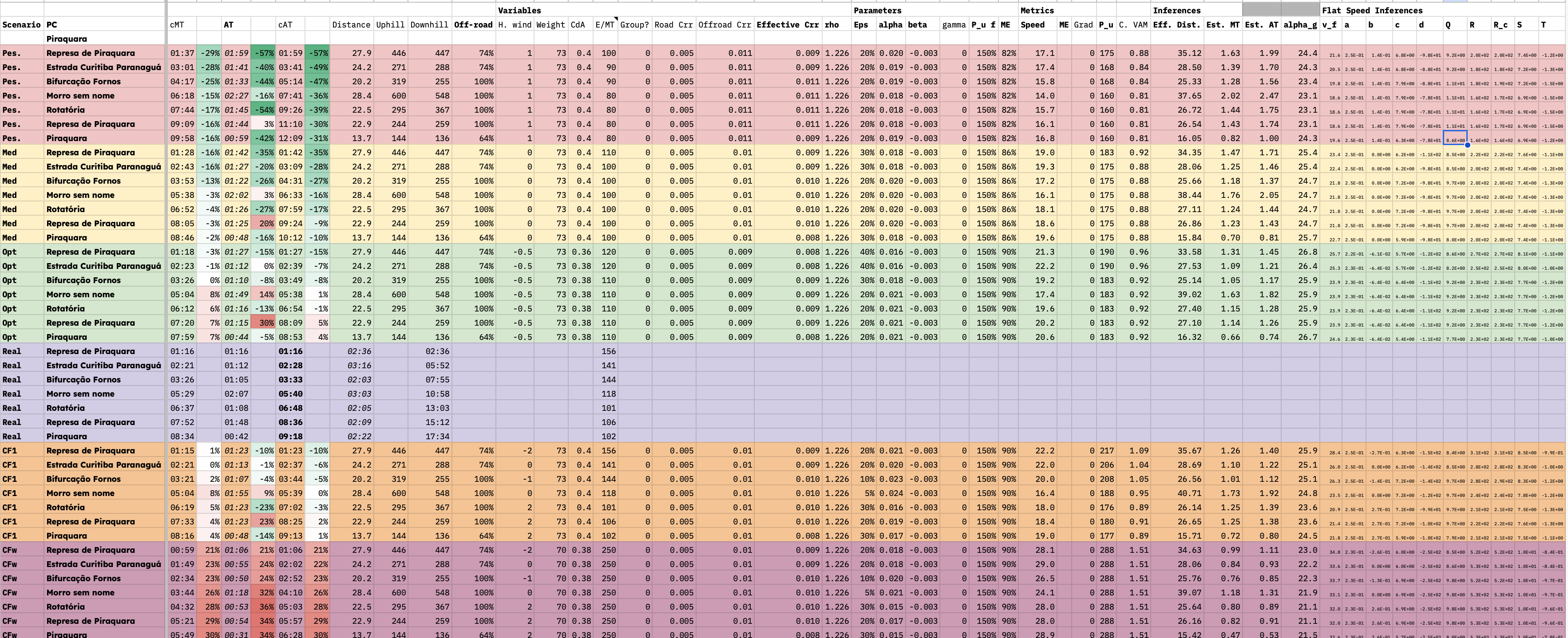
### Predicting and Analyzing outcomes: Gravellands 2023

*Fig: Table containing predicted moving and elapsed times across ex-ante scenarios as well as counterfactual ex-post calibrated scenarios for the Gravellands event*

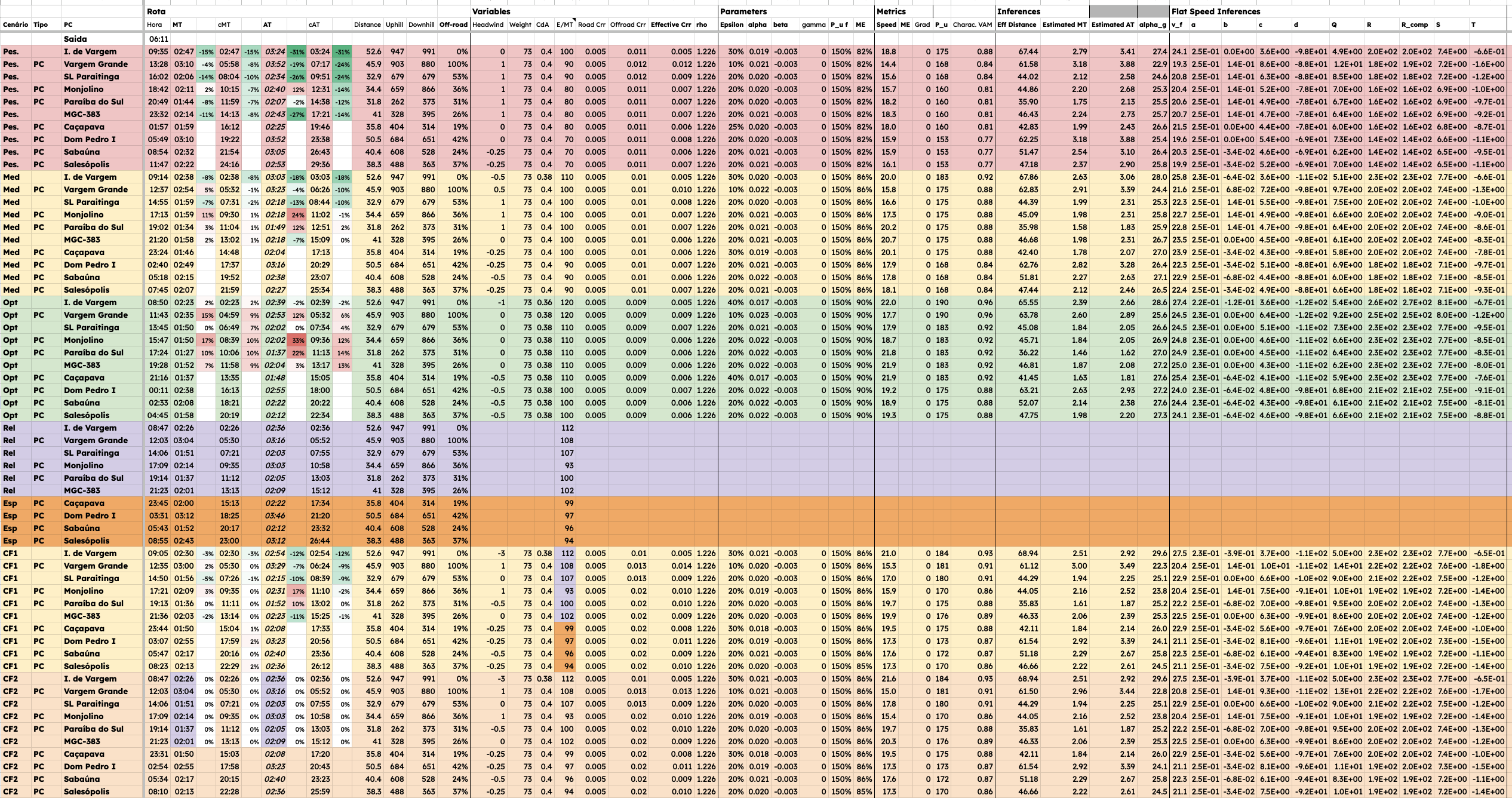
\subsection{Predicting and Analyzing outcomes: RMC400 Salesópolis 2023}

*Fig: Table containing predicted moving and elapsed times across ex-ante scenarios as well as counterfactual ex-post calibrated scenarios for the RMC400 event*

## Conclusions

## References