# **Algorithm 演算法排序筆記**
**[此筆記的原始碼](https://hackmd.io/vopCr9NXTlC4x3DQbWyR2A?both)**
---
## 時間複雜度(Time complexity) $O(f(n))$
定義$T(n)$表示程式執行所要花費的時間，$n$代表資料輸入量。
$O(f(n))$可被視為某演算法在電腦執行所需時間不會超過某一常數倍的$f(n)$，也就是說當某演算法所需的執行時間為$T(n)$，那其時間複雜度為$O(f(n))$。
以數學式表示:
${\exists}c,n_0{\in}constant$,
if $n{\geq}n_0$, then $T(n){\leq}c\cdot f(n)$
所估出來的函數式真正所需執行的上限。
* >Example:假如執行時間為$T(n)=3n^3+2n^2+5n$，求其時間複雜度為何?
Sol:
Find constant $c$ and $n_0$: $(n_0,c)=(0,10)$
when $n{\geq}n_0$,$3n^3+2n^2+5n{\leq}10n^3$, therefore the time complexity is $O(n^3)$

### 常見的Big-O有下列幾種:
| Big O | feature and explanation |
|:------------:|:---------------------------------------------- |
| $O(1)$ | constant time，執行時間為一個常數倍 |
| $O(n)$ | linear time，執行時間會隨資料大小而線性成長 |
| $O(log_2n)$ | sub-linear time，成長速度較線性慢 |
| $O(n^2)$ | quadratic-time，執行時間會成二次方增長 |
| $O(n^3)$ | cubic-time，執行時間會成三次方增長 |
| $O(2^n)$ | exponential time，執行時間會成2的n次方增長 |
| $O(nlog_2n)$ | 線性乘對數時間，介於線性及二次方成長之間的行為 |


## 排序演算法
* 氣泡排序法(Bubble sort)
* 選擇排序法(Selection sort)
* 插入排序法(Insertion sort)
* 希爾排序法(Shell sort)
* 合併排序法(Merge sort)
* 快速排序法(Quick sort)
* 基數排序法(Radix sort)
* 堆積排序法(Heap sort)
### **氣泡排序法(Bubble Sort)**
#### 從第一個元素開始，比較相鄰元素大小，如果順序有誤，則對調再進行下一個元素的比較。掃描過一次後就可以確保最後一個元素是位於正確的位置。接著再進行第二次掃描，直到所有元素完成排序為止。
#### 時間複雜度:
* Best Case: $O(n)$
當資料的順序恰好由小到大時，第一次掃描後，沒有進行任何swap $\Rightarrow$ 提前結束
* Worst Case: $O(n^2)$
當資料的順序恰好為由大到小時，每回合分別執行:$n-1、n-2、...、1$次
因此$(n-1)+(n-2)+...+1=n\cdot\frac{(n-1)}{2}$ $\Rightarrow$ $O(n^2)$
* Average Case: $O(n^2)$
每個數字要執行的次數為$0、1、2、3、...、n-1$，因此每個數字平均的執行次數是$\frac{0+1+2+3+...+(n-1)}{n}=\frac{(n-1)}{2}$，有$n$個數字，所以所需平均時間為$n\cdot\frac{(n-1)}{2}=\frac{(n^2-n)}{2}$ $\Rightarrow$ $O(n^2)$

#### 空間複雜度:
* 不需要額外的陣列去存資料，因此為$\theta(1)$
#### python code:

def bubbleSort(array):
    for i in range(len(array)-1):
        for j in range(0,len(array)-i-1):
            if array[j]>array[j+1]:
                #swap the element
                array[j],array[j+1]=array[j+1],array[j]
    return array

code:https://github.com/coherent17/algorithm/blob/main/sorting/bubblesort.py
#### C code:

#include <stdio.h>
#define SIZE 8

void bubbleSort(int *);
void printArray(int *);
int main(){
	int data[SIZE]={16,25,39,27,12,8,45,63};
	bubbleSort(data);
	printArray(data);
	return 0;
}

void bubbleSort(int *array){
	void swap(int *, int *);
	int i,j;
	for(i=0;i<SIZE-1;i++){
		for(j=0;j<SIZE-1-i;j++){
			if (array[j]>array[j+1]){
				swap(&array[j],&array[j+1]);
			}
		}
	}
} 

void swap(int *a, int *b){
	int temp;
	temp=*a;
	*a=*b;
	*b=temp;
}

void printArray(int *array){
	int i;
	for(i=0;i<SIZE;i++){
		printf("%d ",array[i]);
	}
}

code:https://github.com/coherent17/algorithm/blob/main/sorting/bubblesort.c
#### 改良Bubble Sort (Modified Bubble Sort)
Bubble Sort的時間複雜度只有在給定的陣列為從小到大排序好的情形才會是$O(n)$，其餘情況階是維持$O(n^2)$。因此我們使用一個flag變數去停止bubble sort當陣列已經被排序好了。 初始化flag為True，當有元素進行交換時，flag改為False，當進行完整個迴圈後，若flag還是維持True，則表示該陣列已經被排序好了，便可以停止bubble sort了。
#### python code:

def Modified_bubbleSort(array):
    for i in range(len(array)-1):
        flag=True
        for j in range(0,len(array)-i-1):
            if array[j]>array[j+1]:
                #swap the element and let flag become false
                array[j],array[j+1]=array[j+1],array[j]
                flag=False

                if flag==True:
                    break
    return array

code:https://github.com/coherent17/algorithm/blob/main/sorting/bubblesort.py

#### C code:

#include <stdio.h>
#define SIZE 8

void Modified_bubbleSort(int *);
void printArray(int *);

int main(){
	int data[SIZE]={16,25,39,27,12,8,45,63};
	Modified_bubbleSort(data);
	printArray(data);
	return 0;
}

void Modified_bubbleSort(int *array){
	void swap(int *, int *);
	int i,j,flag;
	for(i=0;i<SIZE-1;i++){
		flag=1;
		for(j=0;j<SIZE-1-i;j++){
			if(array[j]>array[j+1]){
				swap(&array[j],&array[j+1]);
				flag=0;
				if(flag) break;
			}
		}
	}
}

void swap(int *a, int *b){
	int temp;
	temp=*a;
	*a=*b;
	*b=temp;
}

void printArray(int *array){
	int i;
	for(i=0;i<SIZE;i++){
		printf("%d ",array[i]);
	}
}

code:https://github.com/coherent17/algorithm/blob/main/sorting/bubblesort.c
### **選擇排序法(Selection Sort)**
#### 將資料分成已排序及未排序兩部分，依序在未排序中找最小值，加入到已排序部分的末端。按照這個方式，可以在第一輪中找到最小的，第二輪找到第二小的。那要如何從未排序的數列中找到最小值呢?可以先設未排序陣列的第一個數字是目前的最小值，然後再往後一個一個比大小，如果後面的數字比目前的最小值小，那就將目前的最小值換為這個數。
#### 時間複雜度:
分成兩個步驟討論:
* 從未排序陣列中取得最小值:
##### 在n個未排序數列中找到最小值需要$n$個步驟，因此對於selection sort而言，第一回合要從$n$個未排序數列中找到最小值需要$n$個步驟，第二回合要從$n-1$個未排序數列中找到最小值需要$n-1$個步驟，一直到最後一個回合需要一個步驟為止。因此總步驟數為$(n+(n-1)+(n-2)+...+1)=\frac{n\cdot(n+1)}{2}$。
* 移到已排序陣列末端:
##### 每次找到最小的數值，將其與未排序好的第一個數字交換位置，每一個回合需要一個步驟，總共執行$n$個回合，需要$n$個步驟。

因此selection sort共需要$\frac{n\cdot(n+1)}{2}+n=\frac{n\cdot(n+3)}{2}$ $\Rightarrow$ $O(n^2)$

#### 空間複雜度:
* 不需要額外的陣列去存資料，因此為$\theta(1)$
#### python code:

def selectionSort(array):
    for i in range(len(array)-1):
        #設未排序陣列中的第一個元素為最小的
        min_index=i
        for j in range(i+1,len(array)):
            #找到未排序中最小元素的index
            if array[min_index]>array[j]:
                min_index=j
        #將最小的數字放到已排序數列中的最後面
        array[i],array[min_index]=array[min_index],array[i]
    return array

code:https://github.com/coherent17/algorithm/blob/main/sorting/selection_sort.py

#### C code:

#include <stdio.h>
#define SIZE 8

void selectionSort(int *);
void printArray(int *);

int main(){
	int data[SIZE]={16,25,39,27,12,8,45,63};
	selectionSort(data);
	printArray(data);
	return 0;
}

void selectionSort(int *array){
	void swap(int *,int *);
	int i,j,min_index;
	for(i=0;i<SIZE-1;i++){
		//initiaize the index of the unsorted array
		min_index=i;
		
		//find the smallest nuber in the unsorted array
		for(j=i+1;j<SIZE;j++){
			if(array[min_index]>array[j]){
				min_index=j;
			}
		}
		
		//put the smallest number into the last of the sorted array
		swap(&array[min_index],&array[i]);
	}
}

void swap(int *a, int *b){
	int temp;
	temp=*a;
	*a=*b;
	*b=temp;
}

void printArray(int *array){
	int i;
	for(i=0;i<SIZE;i++){
		printf("%d ",array[i]);
	}
}

code:https://github.com/coherent17/algorithm/blob/main/sorting/selectionsort.c

### **插入排序法(Insertion Sort)**
#### 想像手上又一副撲克牌，想要將其由小到大排序。可以將第$i$張牌加入前$i-1$張以排序過的牌，那就可以獲得$i$張排序過的牌組了。
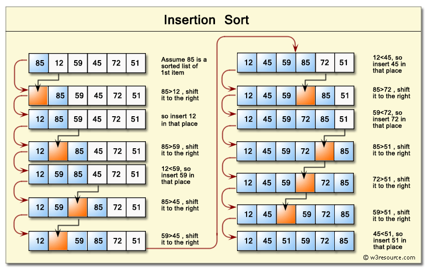
#### 時間複雜度:
* Best Case: $O(n)$
當處理的資料為$1、2、3、4、...、N$時，僅需比較$N$次便可以完成排序。另一方面也表示，當給定的數列已經接近排序的狀態時，用insertion sort效率會很高。
* Worst Case: $O(n^2)$
當處理的資料為顛倒的順序:$N、N-1、N-2、...、2、1$時，那麼位在第$i$個的數字將會需要比較$i-1$次，因此總步驟數為$0+1+2+...+(N-1)=\frac{n\cdot(n-1)}{2}$ $\Rightarrow O(n^2)$
* Average Case: $O(n^2)$
這個好難，之後再來搞懂他，如[連結](http://home.cse.ust.hk/faculty/golin/COMP271Sp03/Notes/Ins_Sort_Average_Case.pdf)
#### 空間複雜度:
* 不需要額外的陣列去存資料，因此為$\theta(1)$
#### python code:

def insertionSort(array):
    for i in range(1,len(array)):
        insert_num=array[i]  #要插入的數字
        j=i-1

        while(j>=0 and insert_num<array[j]):
            array[j+1]=array[j]  #往右移
            j-=1  

        array[j+1]=insert_num  #插入新值
    return array

code:https://github.com/coherent17/algorithm/blob/main/sorting/insertion_sort.py

#### C code:

#include <stdio.h>
#define SIZE 8

void insertionSort(int *);
void printArray(int *);

int main(){
	int data[SIZE]={16,25,39,27,12,8,45,63};
	insertionSort(data);
	printArray(data);
	return 0;
}

void insertionSort(int *array){
	int i,j,insertion_num;
	for(i=1;i<SIZE;i++){
		//the number to insert
		insertion_num=array[i];
		j=i-1;
		
		//shift the number right if the sorted array is bigger than the insertion number
		while(j>=0&&insertion_num<array[j]){
			array[j+1]=array[j];
			j-=1;
		}
		
		//insert the number
		array[j+1]=insertion_num;
	}
}

void printArray(int *array){
	int i;
	for(i=0;i<SIZE;i++){
		printf("%d ",array[i]);
	}
}

code:https://github.com/coherent17/algorithm/blob/main/sorting/insertionsort.c

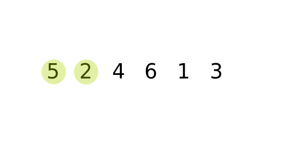
說明:以$array=[5,2,4,6,1,3]$為例。
* 當$i=1\cap j=0$時，我們將$2$這張牌抽出並決定要插在哪裡。此時因為$array[i]<array[j]$，因此將$5$往右挪一格$(array[j+1]=array[j])$，再將比較的值$(array[i])$插入挪出來的位置。此時數列會變成$array=[2,5,4,6,1,3]$
* 當$i=2\cap j=1$時，我們將$4$這張牌抽出並決定要插在哪裡。此時因為$array[i]<array[j]$，因此我們再把$5$往右移一格，將$4$插入挪出來的空格，此時數列會變成$array=[2,4,5,6,1,3]$
* 當$i=3\cap j=2、1、0$時，將$6$這張牌抽出，發現前面的人都比他小，因此不會進入到$while$的迴圈中，維持在原位。此時數列仍然維持$array=[2,4,5,6,1,3]$不變。
* 當$i=4\cap j=3、2、1、0$時，可以發現$1$都比前面的數字還要小，因此將前面的數字依序往後挪一格，再將$1$插入空位，此時數列會變成$array=[1,2,4,5,6,3]$
* 當$i=5\cap j=4、3、2$時，將$3$這張牌抽出，按照前面的規則可以知道將其插入在數字$2$及數字$4$之間，那做到這邊我們就完成我們的排序了，此時數列會變成$array=[1,2,3,4,5,6]$
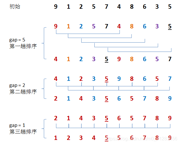
### **希爾排序法(Shell Sort)**
#### 為進化版的插入排序法，改良insertion sort中每次只能將資料移動一位的缺點，因此能夠使原本距離較遠的數字快速歸位。添加了間距(gap)的觀念，往左邊間距gap的數字比大小，可讓在陣列後端數值較小的數字較快回到陣列前端。

#### 舉例說明:有$15$筆資料，取$gap$分別為$5、2、1$
| 0 | 1 | 2 | 3 | 4 | 5 | 6 | 7 | 8 | 9 | 10 | 11 | 12 | 13 | 14 |
| --- | --- |:--- | --- | --- |:--- | --- | --- |:--- |:--- | --- | --- | --- | --- |:--- |
| 45 | 84 | 77 | 83 | 55 | 49 | 91 | 64 | 91 | 5 | 37 | 31 | 70 | 38 | 51 |
* 第一回合: $gap=5$
* 對$index$為$0、5、10$做insertion sort
Example:
| 0 | 1 | 2 | 3 | 4 | 5 | 6 | 7 | 8 | 9 | 10 | 11 | 12 | 13 | 14 |
| ------------------ |:--- |:--- | --- | --- |:----------------- | --- | --- |:--- |:--- | ----------------- | --- | --- | --- |:--- |
| $\color{red} {45}$ | 84 | 77 | 83 | 55 | $\color{red}{49}$ | 91 | 64 | 91 | 5 | $\color{red}{37}$ | 31 | 70 | 38 | 51 |
* 排序後:
| 0 | 1 | 2 | 3 | 4 | 5 | 6 | 7 | 8 | 9 | 10 | 11 | 12 | 13 | 14 |
| ------------------ |:--- |:--- | --- | --- |:----------------- | --- | --- |:--- |:--- | ----------------- | --- | --- | --- |:--- |
| $\color{red} {37}$ | 84 | 77 | 83 | 55 | $\color{red}{45}$ | 91 | 64 | 91 | 5 | $\color{red}{49}$ | 31 | 70 | 38 | 51 |

* 對$index$為$1、6、11$做insertion sort
* 對$index$為$2、7、12$做insertion sort
* 對$index$為$3、8、13$做insertion sort
* 對$index$為$4、9、14$做insertion sort

經過上面$gap=5$的insertion sort後可以發現顏色相同的數組已經按照順序排好了。
| 0 | 1 | 2 | 3 | 4 | 5 | 6 | 7 | 8 | 9 | 10 | 11 | 12 | 13 | 14 |
| ----------------- |:------------------ |:-------------------:| --------------------- |:------------------:|:-----------------:| ------------------ |:-------------------:|:---------------------:|:------------------- |:-----------------:| ------------------ | ------------------- | --------------------- |:------------------- |
| $\color{red}{37}$ | $\color{blue}{31}$ | $\color{green}{64}$ | $\color{magenta}{38}$ | $\color{Brown}{5}$ | $\color{red}{45}$ | $\color{blue}{84}$ | $\color{green}{70}$ | $\color{magenta}{83}$ | $\color{Brown}{51}$ | $\color{red}{49}$ | $\color{blue}{91}$ | $\color{green}{77}$ | $\color{magenta}{91}$ | $\color{Brown}{55}$ |

* 第二回合: $gap=2$
* 將$gap$減至$2$，分成兩組進行insertion sort:
| 0 | 1 | 2 | 3 | 4 | 5 | 6 | 7 | 8 | 9 | 10 | 11 | 12 | 13 | 14 |
| ----------------- | ------------------ |:----------------- | ------------------ | ---------------- |:------------------ | ----------------- | ------------------ |:----------------- |:------------------ | ----------------- | ------------------ | ----------------- | ------------------ |:-----------------:|
| $\color{red}{37}$ | $\color{blue}{31}$ | $\color{red}{64}$ | $\color{blue}{38}$ | $\color{red}{5}$ | $\color{blue}{45}$ | $\color{red}{84}$ | $\color{blue}{70}$ | $\color{red}{83}$ | $\color{blue}{51}$ | $\color{red}{49}$ | $\color{blue}{91}$ | $\color{red}{77}$ | $\color{blue}{91}$ | $\color{red}{55}$ |
* 排序後:
| 0 | 1 | 2 | 3 | 4 | 5 | 6 | 7 | 8 | 9 | 10 | 11 | 12 | 13 | 14 |
| ----------------- | ------------------ |:----------------- | ------------------ | ---------------- |:------------------ | ----------------- | ------------------ |:----------------- |:------------------ | ----------------- | ------------------ | ----------------- | ------------------ |:-----------------:|
| $\color{red}{5}$ | $\color{blue}{31}$ | $\color{red}{37}$ | $\color{blue}{38}$ | $\color{red}{49}$ | $\color{blue}{45}$ | $\color{red}{55}$ | $\color{blue}{51}$ | $\color{red}{64}$ | $\color{blue}{70}$ | $\color{red}{77}$ | $\color{blue}{91}$ | $\color{red}{83}$ | $\color{blue}{91}$ | $\color{red}{84}$ |
可以看出顏色相同的數組已經被由小到大排序好了，此外，也可以看到較小的數字已經都在左側，而較大的數字也都已經移到右側了，已經變成一個快要完全排序完成的數列了，此時我們可以進行$gap=1$的排序，其實也就是前面所介紹的insertion sort，在這種快要排序好的數列中，insertion sort的效能會是很高的。

* 第三回合: $gap=1$，其實就是前面所說的insertion sort，只不過這邊不分組，是將所有數列一起做一次insertion sort，便可以得到最終排序好的數列。
* 排序後:
| 0 | 1 | 2 | 3 | 4 | 5 | 6 | 7 | 8 | 9 | 10 | 11 | 12 | 13 | 14 |
| --- | --- |:--- | --- | --- |:--- | --- | --- |:--- |:--- | --- | --- |:---:| --- |:--- |
| 5 | 31 | 37 | 38 | 45 | 49 | 51 | 55 | 64 | 70 | 77 | 83 | 84 | 91 | 91 |


**好懂的示意影片**:{%youtube CmPA7zE8mx0 %}
#### 時間複雜度:
* 依step的不同而有不同的時間複雜度，但是仍快於insertion sort
#### python code:

data=[45,84,77,83,55,49,91,64,91,5,37,31,70,38,51]
#define the gap by yourself
gap=[5,2,1]

def shell_sort(array,gap):
    n=len(array)
    #start gapped insertion sort
    for current_gap in gap:
        for i in range(current_gap,n):
            #temp: the insertion number
            temp=array[i]
            j=i
            #if the unsorted array is bigger than insertion number, then shift right 
            while j>=0 and j-current_gap>=0 and array[j-current_gap]>temp:
                array[j]=array[j-current_gap]
                j-=current_gap
            #insert the insertion number
            array[j]=temp
    return array

code:https://github.com/coherent17/algorithm/blob/main/sorting/shell_sort.py

#### C code:

#include <stdio.h>
#define SIZE 15

void shellSort(int *, int *);
void printArray(int *);

int main(){
	int data[SIZE]={45,84,77,83,55,49,91,64,91,5,37,31,70,38,51};
	//define gap by yourself
	int gap[3]={5,2,1};
	shellSort(data,gap);
	printArray(data);
	return 0;
}

void shellSort(int *array, int *gap){
	int i,j,k,current_gap,temp;
	for(i=0;i<3;i++){
		current_gap=gap[i];
		for(j=current_gap;j<SIZE;j++){
			temp=array[j];
			k=j;
			while(k>=0&&k-current_gap>=0&&array[k-current_gap]>temp){
				array[k]=array[k-current_gap];
				k-=current_gap;
			}
			array[k]=temp;
		}
	}
}

void swap(int *a, int *b){
	int temp;
	temp=*a;
	*a=*b;
	*b=temp;
}

void printArray(int *array){
	int i;
	for(i=0;i<SIZE;i++){
		printf("%d ",array[i]);
	}
}

code:https://github.com/coherent17/algorithm/blob/main/sorting/shellsort.c
### **合併排序法(Merge Sort)**
#### 分治法(Divide-and-conquer):
在進入合併排序法前，我們先來看看分治法:把一個複雜的問題分成兩個或更多的相同或相似的子問題，直到最後子問題可以簡單的直接求解，原問題的解即子問題的解的合併。
在紙房子(一)第11集中，教授有預期警方會透過這種分治法去一一擊破夥伴們的心理，因此有事先想好應對的策略!

#### 合併排序法大致上可以分為切分與排序
* 切分:
* 1.將原陣列切一半成兩個子陣列
* 2.將切好的子陣列再切一半
* 3.重複第2步直到所有子陣列只包含一個元素
* 排序:
* 1.排序兩個只剩一個元素並合併為一個陣列
* 2.將兩邊排序好的陣列再合併為一個陣列
* 3.重複2直到所有陣列合併為一個大陣列

#### 舉例說明:
* 
* 因為兩個子陣列在合併前是已經排序好的狀態，因此在合併兩個已排序後的陣列，我們僅需持續比較最前面最小的部分，再將較小的丟到新的大陣列即可，便可以完成排序。

#### 時間複雜度:
* 切分:
* 將一個長度為$n$的陣列切為每個子陣列長度為1需要$n-1$個步驟
* 合併&排序:
* 將兩個排序好的子陣列(長度和為$n$)合併為排序好的大陣列需要$n$個步驟(兩個子陣列的最前的元素來比較)，那在merge sort中需要執行幾次這樣的合併步驟呢?假設一開始有8個子陣列合併成4個，再合併為2個，最後合併為一個，因此需要執行$log_2n$次，因此再合併與排序的步驟數為$nlog_2n$
* 結合切分與合併:
* 合併的總步驟數為$(n-1)+(nlog_2n)$，因此merge sort的時間複雜度為$O(nlog_2n)$

#### 空間複雜度:
* 假設原未排序的陣列長度為$n$，需要額外的$n$長度的陣列來儲存已排序的陣列，引此空間複雜度為$\theta(n)$

#### python code(divide and conquer):
* 1.申請空間，使其大小為兩個已經排序序列之和，該空間用來存放合併後的序列
* 2.設定兩個指標，最初位置分別為兩個已經排序序列的起始位置
* 3.比較兩個指標所指向的元素，選擇相對小的元素放入到合併空間，並移動指標到下一位置
* 4.重複步驟3直到某一指標到達序列尾
* 5.將另一序列剩下的所有元素直接複製到合併序列尾

def merge_sort(array):
    if len(array)>1:
        #find the division point
        mid=len(array)//2
        left_array=array[:mid]
        right_array=array[mid:]

        #use recursion to keep dividing
        merge_sort(left_array)
        merge_sort(right_array)

        #initialize the comparison index
        right_index=0
        left_index=0
        merge_index=0

        #start comparing
        #case 1: right array compare with left array
        while right_index<len(right_array) and left_index<len(left_array):
            if right_array[right_index]<left_array[left_index]:
                array[merge_index]=right_array[right_index]
                right_index+=1
            else:
                array[merge_index]=left_array[left_index]
                left_index+=1
            merge_index+=1
        
        #case 2: right array compare with itself
        while right_index<len(right_array):
            array[merge_index]=right_array[right_index]
            right_index+=1
            merge_index+=1
        
        #case 3: left array compare with itself
        while left_index<len(left_array):
            array[merge_index]=left_array[left_index]
            left_index+=1
            merge_index+=1
    return array

code:https://github.com/coherent17/algorithm/blob/main/sorting/merge_sort.py

#### C code:

#include <stdio.h>
#define SIZE 8 

void mergeSort(int *, int *, int, int);
void printArray(int *);

int main(){
	int data[SIZE]={5,3,8,6,2,7,1,4};
	int reg[SIZE]={0};
	mergeSort(data,reg,0,SIZE-1);
	printArray(data);
	return 0;
}

void mergeSort(int *array, int *reg, int front, int end){
	int mid;	
	if(front<end){
		mid=(front+end)/2;
		//left sub-array:array[front,...,mid]
		//right sub-array:array[mid+1,...,end]
		mergeSort(array,reg,front,mid);
		mergeSort(array,reg,mid+1,end);
		
		//initialize the comparison pointer
		int left_pointer=front;
		int right_pointer=mid+1;
		
		//loop counter
		int i;
		
		for(i=front;i<=end;i++){
			//limit of the left pointer
			if(left_pointer==mid+1){
				reg[i]=array[right_pointer];
				right_pointer+=1;
			}
			
			//limit of the right pointer
			else if(right_pointer==end+1){
				reg[i]=array[left_pointer];
				left_pointer+=1;
			}
			
			//the element of the left sub-array is smaller than right sub-array
			else if(array[left_pointer]<array[right_pointer]){
				reg[i]=array[left_pointer];
				left_pointer+=1;
			}
			
			//the element of the right sub-array is smaller than left sub-array
			else{
				reg[i]=array[right_pointer];
				right_pointer+=1;
			}
		}
		
		//copy the element from register to array
		for(i=front;i<=end;i++){
			array[i]=reg[i];
		}
	}
}

void printArray(int *array){
	int i;
	for(i=0;i<SIZE;i++){
		printf("%d ",array[i]);
	}
}

code:https://github.com/coherent17/algorithm/blob/main/sorting/mergesort.c

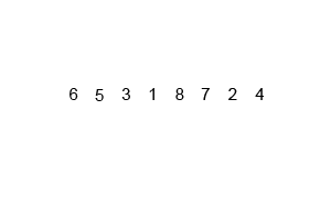
### **快速排序法(Quick Sort)**
#### 找到一個基準點(pivot)，將比這個基準點小的元素放至左邊的子陣列，將比這個基準點大的元素放到右邊的子陣列，如此一來便能確定這個基準點的位置會是最終排序過後正確的位置，再對左邊的子陣列與右邊的子陣列重複進行相同的步驟，便能完成排序。

#### 舉例說明:
Note:此處pivot的選擇為要排序陣列的最後一個元素
$i$要找的是比pivot大的元素，而$j$要找的是比pivot小的元素。
| $\downarrow$ i | | | | | | | $\downarrow$ p |
| -------------- | --- |:---:|:---:|:---:| --- |:----------------:|:---------------:|
| 22 | 11 | 88 | 66 | 55 | 77 | 33 | 44 |
| | | | | | | $\uparrow$ **j** | |

$i$往右移，直到找到比pivot數值還要大的元素便停止:

| | $\downarrow$ i | | | | | | $\downarrow$ p |
|:---:| -------------- |:---:|:---:|:---:| --- |:----------------:|:---------------:|
| 22 | 11 | 88 | 66 | 55 | 77 | 33 | 44 |
| | | | | | | $\uparrow$ **j** | |

| | | $\downarrow$ i | | | | | $\downarrow$ p |
|:---:| --- |:--------------:|:---:|:---:|:---:|:----------------:|:---------------:|
| 22 | 11 | 88 | 66 | 55 | 77 | 33 | 44 |
| | | | | | | $\uparrow$ **j** | |

$j$往左移，直到找到比pivot數值還要小的元素便停止:

| | | $\downarrow$ i | | | | | $\downarrow$ p |
|:---:| --- |:--------------:|:---:|:---:|:---:|:----------------:|:---------------:|
| 22 | 11 | 88 | 66 | 55 | 77 | 33 | 44 |
| | | | | | | $\uparrow$ **j** | |

而後將陣列中$index$為$i$與$j$的元素對調:

| | | $\downarrow$ i | | | | | $\downarrow$ p |
|:---:| --- |:--------------:|:---:|:---:|:---:|:----------------:|:---------------:|
| 22 | 11 | 33 | 66 | 55 | 77 | 88 | 44 |
| | | | | | | $\uparrow$ **j** | |

持續進行上面的步驟直到$i < j$:
($i$往右移找比pivot大的，$j$往左移找比pivot小的)

| | | | $\downarrow$ i | | | | $\downarrow$ p |
|:---:| --- |:----------------:|:--------------:|:---:|:---:|:---:|:---------------:|
| 22 | 11 | 33 | 66 | 55 | 77 | 88 | 44 |
| | | $\uparrow$ **j** | | | | | |

而後將陣列中$index$為$i$與$p$的元素對調:

| 22 | 11 | 33 | $\color{green}{44}$ | 55 | 77 | 88 | 66 |
|:---:| --- |:----------------:|:-------------------:|:---:|:---:|:---:|:---------------:|

此時已經可以確定最開始時設定的pivot位置對於最終排序好的陣列是不會再改變了，而且在pivot左邊的子陣列中的元素都比它小，而pivot右邊的子陣列中的元素都比它大。未來僅需對pivot左邊的子陣列及右邊的子陣列同樣進行上述的步驟，便可以得到排序好的陣列!

對於左邊的子陣列持續進行上面同樣的步驟直到$i < j$:
($i$往右移找比pivot大的，$j$往左移找比pivot小的)

| $\downarrow$ i | | $\downarrow$ p | | | | | |
|:--------------:| ---------------- |:---------------:|:-------------------:|:---:|:---:|:---:|:---:|
| 22 | 11 | 33 | $\color{green}{44}$ | 55 | 77 | 88 | 66 |
| | $\uparrow$ **j** | | | | | | |

| | | $\downarrow$ i $\downarrow$ p | | | | | |
|:---:| ---------------- |:-------------------------------:|:-------------------:|:---:|:---:|:---:|:---:|
| 22 | 11 | 33 | $\color{green}{44}$ | 55 | 77 | 88 | 66 |
| | $\uparrow$ **j** | | | | | | |

而後將陣列中$index$為$i$與$p$的元素對調:
(剛好是同一個元素，位置不動)
| 22 | 11 | $\color{green}{33}$ | $\color{green}{44}$ | 55 | 77 | 88 | 66 |
|:---:| --- |:-------------------:|:-------------------:|:---:|:---:|:---:|:---:|

繼續對左邊的子陣列進行一樣的步驟:

| $\downarrow$ i | $\downarrow$ p | | | | | | |
|:----------------:|:---------------:|:-------------------:|:-------------------:|:---:|:---:|:---:|:---:|
| 22 | 11 | $\color{green}{33}$ | $\color{green}{44}$ | 55 | 77 | 88 | 66 |
| $\uparrow$ **j** | | | | | | | |

此時可以發現$i$與$j$為同一個元素，直接判斷此元素是否比pivot大，若有將陣列中$index$為$i$與$p$的元素對調，若否，則維持不動。

| $\color{green}{11}$ | $\color{green}{22}$ | $\color{green}{33}$ | $\color{green}{44}$ | 55 | 77 | 88 | 66 |
|:-------------------:| ------------------- |:-------------------:|:-------------------:|:---:|:---:|:---:|:---:|

我們就完成左半邊陣列的排序了，接著對陣列右半邊以同樣的步驟進行排序，最後變可以成功地得到已排序的陣列:

| $\color{green}{11}$ | $\color{green}{22}$ | $\color{green}{33}$ | $\color{green}{44}$ | $\color{green}{55}$ | $\color{green}{66}$ | $\color{green}{77}$ | $\color{green}{88}$ |
|:-------------------:| ------------------- |:-------------------:|:-------------------:|:-------------------:|:-------------------:|:-------------------:|:-------------------:|

#### 時間複雜度:
* Best Case: $O(nlogn)$
* Worst Case: $O(n^2)$

#### python code(divide and conquer):

data=[22,11,88,66,55,77,33,44]

def quicksort(array,left,right):
    if left<right:
        partition_pos=partition(array,left,right)
        quicksort(array,left,partition_pos-1)
        quicksort(array,partition_pos+1,right)


def partition(array,left,right):
    i=left
    j=right-1
    pivot=array[right]

    while i<j:
        #i move to right:
        while i<right and array[i]<pivot:
            i+=1
        
        #j move to left:
        while j>left and array[j]>pivot:
            j-=1

        #swap the element of index i and j
        if i<j:
            array[i],array[j]=array[j],array[i]

    #swap the element of index i and p
    if array[i]>pivot:
        array[i],array[right]=array[right],array[i]

    return i    

quicksort(data,0,len(data)-1)
print(data)

code:https://github.com/coherent17/algorithm/blob/main/sorting/quicksort.py

#### C code:

#include <stdio.h>
#define SIZE 8

void swap(int *, int *);
int partition(int *, int, int);
void quickSort(int *, int, int);
void printArray(int *);

int main(){
	int data[SIZE]={22,11,88,66,55,77,33,44};
	quickSort(data,0,SIZE-1);
	printArray(data);
	return 0;
}

void quickSort(int *array, int left, int right){
	if(left<right){
		int partition_pos;
		partition_pos=partition(array,left,right);
		quickSort(array,left,partition_pos-1);
		quickSort(array,partition_pos+1,right);
	}
} 

int partition(int *array, int left, int right){
	int i,j,pivot;
	i=left;
	j=right;
	pivot=array[right];
	
	while(i<j){
		//i move to right
		while(i<right&&array[i]<pivot){
			i++;
		}
		//j move to left
		while(j>left&&array[j]>pivot){
			j--;
		}
		//swap the element of the index i and j
		if(i<j){
			swap(&array[i],&array[j]);
		}
	}
	//swap the element of the index i and p
	if(array[i]>pivot){
		swap(&array[i],&array[right]);
	}
	return i;
}

void swap(int *a, int *b){
	int temp;
	temp=*a;
	*a=*b;
	*b=temp;
}

void printArray(int *array){
	int i;
	for(i=0;i<SIZE;i++){
		printf("%d ",array[i]);
	}
}

code:https://github.com/coherent17/algorithm/blob/main/sorting/quicksort.c

### **基數排序法(Radix Sort)**
#### 為一種分配式的排序法(distribution sort)，可以分成LSD或MSD，在不同的情形可以使用不同的方式，使其達到最高效率。在做基數排序法的時候會用到桶子，存放陣列的值。

#### 舉例說明:
以LSD(least significant digit)為例子:

給定義下陣列:
| 73 | 22 | 93 | 43 | 55 | 14 | 28 | 65 | 39 | 81 |
| --- | --- | --- | --- | --- | --- | --- | --- | --- |:---:|

**Step 1:**
在經過這些數值時，依據個位數的大小將其分配到0~9的桶子內，並遵守下面的規則:
* 1.數值存放時要從桶子的底部開始。
* 2.一旦有其中一個桶子放到第$n$層，其餘桶子在分配時也需要從第$n$層開始放。
* ex:73的個位數字為3，將其放到3號桶子的最底部。
* ex:22的個位數字為2，將其放到2號桶子的最底部。
* ex:93的個位數字為3，將其放到3號桶子，但是下面已經有放置73，因此放到第二層。
* ex:43的個位數字為3，將其放到3號桶子，但是下面已經有放置73和93，因此放到第三層。
* ex:55的個位數字為5，但是因3號桶子已經放到第三層，因此將其放到5號桶子的第三層。

按照以上規則，將陣列的所有數值依據個位數排序好之後可以獲得:

| 0 | 1 | 2 | 3 | 4 | 5 | 6 | 7 | 8 | 9 |
| --- |:---:|:---:|:---:| --- |:---:| --- | --- |:---:|:---:|
| | 81 | | | | 65 | | | | 39 |
| | | | 43 | 14 | 55 | | | 28 | |
| | | | 93 | | | | | | |
| | | 22 | 73 | | | | | | |

**Step 2:**
將剛剛依據個位數放進桶子的數值串接起來，並遵守下面的規則:
* 1.由編號0的桶子取到編號9的桶子。
* 2.同一個桶子內，先取放置在底部的。

由以上規則，我們所得到的陣列為:
| 81 | 22 | 73 | 93 | 43 | 14 | 55 | 65 | 28 | 39 |
| --- | --- | --- | --- | --- | --- | --- | --- | --- |:---:|

**Step 3:**
重複Step 1，不過改成對十位數進行分配:
按照以上規則，將陣列的所有數值依據十位數排序好之後可以獲得:

| 0 | 1 | 2 | 3 | 4 | 5 | 6 | 7 | 8 | 9 |
| --- |:---:|:---:|:---:|:---:|:---:|:---:|:---:|:---:|:---:|
| | | 28 | 39 | | | | | | |
| | 14 | 22 | | 43 | 55 | 65 | 73 | 81 | 93 |

**Step 4:**
重複Step 2，將其串接在一起，便完成了排序:
| 14 | 22 | 28 | 39 | 43 | 55 | 65 | 73 | 81 | 93 |
| --- | --- | --- | --- | --- | --- | --- | --- | --- |:---:|

要進行幾次的分配及串接是取決於這些數值中最大位數的那個數字有幾位。

LSD的radix sort適用於位數較少的數列，然而在運算數值較大的陣列則是MSD的radix sort效率會比較高。
#### 時間複雜度:
定義$n$為陣列長度，而$k$為此陣列最大數字的位數。
* Best Case: $O(nk)$
* Worst Case: $O(nk)$

#### python code:

def getMax(array):
    max=array[0]
    for i in range(1,len(data)):
        if array[i]>max:
            max=array[i]
    return max

def radixSort(array):
    temp_array=[0]*len(array)
    significantDigit=1
    largestNum=getMax(array)

    while largestNum/significantDigit>0:
        bucket=[0]*10

        # count how many number put into each bucket
        for i in range(len(array)):
            bucket[int(array[i]/significantDigit)%10]+=1

        # use prefix sum to determine where to put the number 
        for i in range(1,9+1):
            bucket[i]+=bucket[i-1]

        
        for i in range(len(array)-1,-1,-1):
            digitNumber=int(array[i]/significantDigit)%10
            # need to -1 because the prefix sum include itself
            bucket[digitNumber]-=1
            temp_array[bucket[digitNumber]]=array[i]

        # copy the array
        for i in range(len(array)):
            array[i]=temp_array[i]

        significantDigit*=10
    return array

code:https://github.com/coherent17/algorithm/blob/main/sorting/radixort.py

#### C code:

#include <stdio.h>
#define SIZE 8

int getMax(int *);
void radixSort(int *);
void printArray(int *);

int main(){
	int data[SIZE]={170,45,75,90,802,24,2,66};
	radixSort(data);
	printArray(data);
	return 0;
}

int getMax(int *array){
	int max,i;
	max=array[0];
	for(i=1;i<SIZE;i++){
		if(array[i]>max){
			max=array[i];
		}
	}
	return max;
}

void radixSort(int *array){
	int i;
	int temp_array[SIZE];
	int significantDigit=1;
	int largestNum=getMax(array);
	
	while(largestNum/significantDigit>0){
		int bucket[10]={0};
		
		//count how many number put into each bucket
		for(i=0;i<SIZE;i++){
			bucket[(array[i]/significantDigit)%10]++;
		}
		
		//use prefix sum to determine where to put the number 
		for(i=1;i<10;i++){
			bucket[i]+=bucket[i-1];
		}
		
		for(i=SIZE-1;i>=0;i--){
			int digitNumber=(array[i]/significantDigit)%10;
			//need to -1 because the prefix sum include itself
			temp_array[--bucket[digitNumber]]=array[i];
		}
		
		//copy the array
		for(i=0;i<SIZE;i++){
			array[i]=temp_array[i];
		}
		
		//move to the next significantDigit number
		significantDigit*=10;
	}
}

void printArray(int *array){
	int i;
	for(i=0;i<SIZE;i++){
		printf("%d ",array[i]);
	}
} 

code:https://github.com/coherent17/algorithm/blob/main/sorting/radixsort.c
* 解釋程式碼:
* 因為在上面radix sort的解釋中，可以看到若是用二維陣列去存這些數值，其實會浪費許多空間，不如我們可以使用前綴和的技巧，便能成功定位出該數值在串接時應該要被放置的位置，且節省許多不必要空間的使用。

### **推積排序法(Heap Sort)**
在了解堆積排序法前，需要先知道:
* 1.complete binary tree(完全二元樹)
* 2.heap data structure(堆積)

#### complete binary tree(完全二元樹):
* 樹的概念:
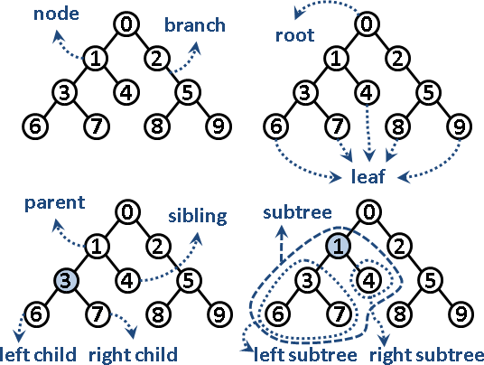
* 二元樹的分類:
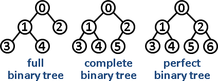
* full binary tree:除了最底層的樹葉以外，其餘節點都有兩個小孩。
* complete binary tree:各層節點全滿，除了最後一層，最後一層節點全部靠左。
* perfect binary tree:各層節點全滿，每個節點都有兩個小孩。

#### heap data structure(堆積):
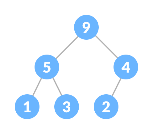
* heap property:
* 1.max heap(最大堆積):所有節點的小孩都比其小，根部為最大值。
example:
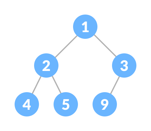
* 2.min heap(最小堆積):所有節點的小孩都比其大，根部為最小值。
example:
* Heapify(堆積化):將二元樹化為最大堆積或是最小堆積的過程。
* 給定陣列(n=6):
| 0 | 1 | 2 | 3 | 4 | 5 |
| --- | --- |:---:| --- | --- |:---:|
| 3 | 9 | 2 | 1 | 4 | 5 |
* 建立complete binary tree:
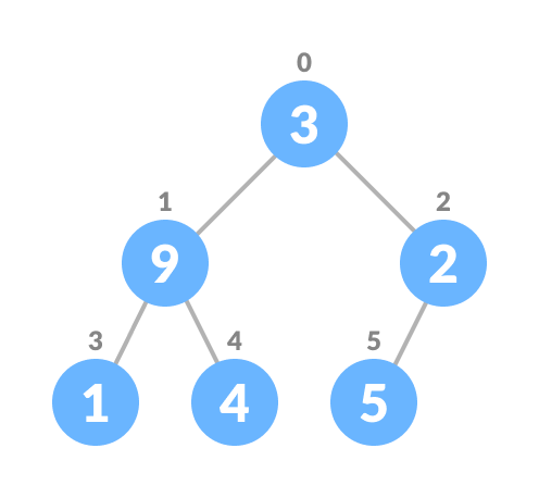
* 從第一個非葉子的節點開始，index為$i=n/2-1=2$，將其設為當前最大值，然後去比較左小孩(index為$2i+1$)及右小孩(index為$2i+2$)，若左小孩或右小孩比當前最大值為大，則將其設為當前最大值，並將其與此時index為$i$的元素交換，持續重複此步驟，直到所有子樹都被堆積完成。
* 在二元樹中加入新的元素:
* 將此元素加在二元樹的末端，再做heapify。
* 在二元樹中刪除元素:
* 將欲刪除的元素移至樹的末端，刪除後再做heapify。

#### C code for max heap data structure:

#include <stdio.h>

void swap(int *, int *);
void heapify(int *, int, int);
void insert(int *, int);
void delete(int *, int);
void printArray(int *, int);

//global variable
int size=0;

int main(){
    int array[10];
    insert(array,3);
    insert(array,4);
    insert(array,9);
    insert(array,5);
    insert(array,2);
    printArray(array,size);
    delete(array,9);
    printArray(array,size);
    return 0;
}

void swap(int *a, int *b){
    int temp;
    temp=*a;
    *a=*b;
    *b=temp;
}

void heapify(int *array, int size, int i){
    int largest=i;
    int left_children=2*i+1;
    int right_children=2*i+2;

    if(left_children<size && array[left_children]>array[largest]) largest=left_children;
    if(right_children<size && array[right_children]>array[largest]) largest=right_children;
    //check need to swap or not?
    if(largest!=i){
        swap(&array[i],&array[largest]);
        heapify(array,size,largest);
    }
}

void insert(int *array, int newNumber){
    array[size]=newNumber;
    size+=1;
    //loop to heapify
    int i;
    for(i=size/2-1;i>=0;i--){
        //i is the index of the parent node
        heapify(array, size, i);
    }
}

void delete(int *array, int delNumber){
    //find the index of the number to delete
    int i;
    for(i=0;i<size;i++){
        if(array[i]==delNumber) break;
    }
    //swap to the end of the binary tree
    swap(&array[i],&array[size-1]);
    size-=1;
    //loop to heapify
    for(i=size/2-1;i>=0;i--){
        heapify(array, size, i);
    }
}

void printArray(int *array,int size){
	int i;
	for(i=0;i<size;i++){
		printf("%d ",array[i]);
	}
    printf("\n");
}

code:https://github.com/coherent17/algorithm/blob/main/sorting/max_heap_data_structure.c
#### Heap sort實踐方法:
那要如何透過堆積的排序數列呢?我們可以將每次heapify後的binary tree的最大值(根部root)，將其與樹的末端交換，也就是將其放到陣列的最後一個位置，之後刪除其在binary tree中的位置，再繼續進行相同的動作便可以將此數列排序完畢。

#### 時間複雜度:
* Best case:$O(nlogn)$
* Worst case:$O(nlogn)$
* Average case:$O(nlogn)$

##### python code:

def heapify(array,size,i):
    largest=i
    left_children=2*i+1
    right_children=2*i+2

    if left_children<size and array[left_children]>array[largest]:
        largest=left_children
    if right_children<size and array[right_children]>array[largest]:
        largest=right_children
    
    # //check need to swap or not?
    if largest!=i:
        array[i],array[largest]=array[largest],array[i]
        heapify(array,size,largest)

def heapSort(array):
    # construct max heap:
    n=len(array)
    for i in range(n//2,-1,-1):
        heapify(array,n,i)
    
    # swap the root(index=0) to the end of the array and delete it
    for i in range(n-1,0,-1):
        array[i],array[0]=array[0],array[i]
        #heapify root element:
        heapify(array,i,0)

code:https://github.com/coherent17/algorithm/blob/main/sorting/heapsort.py
##### C code:

#include <stdio.h>
#define SIZE 8

void swap(int *, int *);
void heapify(int *, int, int);
void heapSort(int *, int);
void printArray(int *);

int main(){
    int data[SIZE]={16,25,39,27,12,8,45,63};
    heapSort(data,SIZE);
    printArray(data);
    return 0;
}
void swap(int *a, int *b){
    int temp;
    temp=*a;
    *a=*b;
    *b=temp;
}

void heapify(int *array, int size, int i){
    int largest=i;
    int left_children=2*i+1;
    int right_children=2*i+2;

    if(left_children<size && array[left_children]>array[largest]) largest=left_children;
    if(right_children<size && array[right_children]>array[largest]) largest=right_children;
    //check need to swap or not?
    if(largest!=i){
        swap(&array[i],&array[largest]);
        heapify(array,size,largest);
    }
}

void heapSort(int *array, int size){
    //construct max heap:
    int i;
    for(i=size/2-1;i>=0;i--){
        heapify(array, size, i);
    }

    //swap the root(index=0) to the end of the array and delete it
    for(i=size-1;i>=0;i--){
        swap(&array[0],&array[i]);
        //heapify again to get the maxheap
        heapify(array,i,0);
    }
}

void printArray(int *array){
	int i;
	for(i=0;i<SIZE;i++){
		printf("%d ",array[i]);
	}
    printf("\n");
}

code:https://github.com/coherent17/algorithm/blob/main/sorting/heapsort.c