---
title: "BeeSeq Project"
author: "Dave Angelini"
affiliation: "Colby College"
date: 2018-03-29
output:
html_document:
css: /Users/drangeli/Documents/3.research/BeeSeq.project/BlackUbuntu.css
highlight: tango
toc: true
toc_float: true
toc_depth: 3
---
> [Main page](https://hackmd.io/s/BJ4FiV_W7)
<a name="top"></a>
# BeeSeq
Dave Angelini
March 29, 2018
| |
|:--:|
| 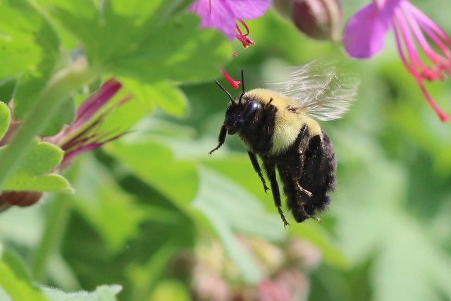 |
| *Bombus impatiens* (photo: [Dave Angelini](https://www.flickr.com/photos/142092478@N03/42829304472)) |
# Microbiome analysis
## 16S v4-v5
Paired-end 2x300bp MiSeq libraries were made by Andre Comeau at the [Dalhousie University IMR](http://cgeb-imr.ca/index.html), from amplicons targetting 16S v4-v5.
* 515F `GTGYCAGCMGCCGCGGTAA`
* 926R `CCGYCAATTYMTTTRAGTTT`
* The product is **410 bp**, resulting in a 190 bp overlap.
> Parada AE, Needham DM, Fuhrman JA. 2016. Every base matters: assessing small subunit rRNA primers for marine microbiomes with mock communities, time series and global field samples. *Environ Microbiol* 18(5):1403-14. [Link](http://dx.doi.org/10.1111/1462-2920.13023)
> Walters W, Hyde ER, Berg-Lyons D, Ackermann G, Humphrey G, Parada A, Gilbert JA, Jansson JK, Caporaso JG, Fuhrman JA, Apprill A, Knight B. 2015. Improved bacterial 16S rRNA gene (V4 and V4-5) and fungal internal transcribed spacer marker gene primers for microbial community surveys. *mSystems* 1(1):e00009-15. [Link](https://msystems.asm.org/content/1/1/e00009-15)
### Data processing
In order to make Qiime work more smoothly, I'll rename the raw data files to have names without any special characters like dashes or underscores.
This can be done with a few variations on...
```bash
rename 1-d 1d ?1-d*
rename d0- d00n ??d0-*
```
Set the Qiime2 docker alias. Note that I updated to the June 2018 Qiime2 release.
```bash
alias qiime 'docker run -t -i -v /export/groups/drangeli/beeSeq.project/16s.v4v5/:/data qiime2/core:2018.6 qiime'
```
Import the data and summarize.
```bash
qiime tools import \
--type 'SampleData[PairedEndSequencesWithQuality]' \
--input-path raw.reads \
--source-format CasavaOneEightSingleLanePerSampleDirFmt \
--output-path 16s.v4.demux.qza
qiime demux summarize \
--i-data 16s.v4.demux.qza \
--o-visualization 16s.v4.demux.qzv
```
I ran the dada2 denoise process under a range of truncation parameters using a bash script to run the denoise command and produce a `feature.table.qza` and `tsv` file. I used the total number of features (presumptive OTUs) as the metric to choose.

The parameters that produce the maximum number of features are `--p-trunc-len-f 260 --p-trunc-len-r 175`, corresponding to a quality score cutoff of roughly 34 as seen in the quality plot in the `16s.v4.demux.qzv` file.
```bash
qiime dada2 denoise-paired \
--i-demultiplexed-seqs 16s.v4.demux.qza \
--p-trunc-len-f 260 --p-trunc-len-r 175 \
--p-trim-left-f 34 --p-trim-left-r 34 \
--o-representative-sequences 16s.v4.rep.seqs.qza \
--o-table 16s.v4.feature.table.qza \
--o-denoising-stats 16s.v4.denoise.stats.qza \
--p-n-threads 16
```
Export the feature table to a format that can be read by R.
```bash
qiime tools export \
16s.v4.feature.table.qza \
--output-dir .
docker run -t -i -v /export/groups/drangeli/beeSeq.project/16s.v4v5/:/data qiime2/core:2018.6 \
biom convert \
-i feature-table.biom \
-o 16s.v4.feature.table.tsv \
--to-tsv
```
The resulting tab-separated values (tsv) file is a table of counts for each feature in each sample. This can be imported into R for custom statistical tests, plots, or other analyses. The features in this table are named by their UUIDs, but their taxonomy assignments can be matched up to the ID using `16s.v4.taxonomy.tsv`, which is generated later in this workflow.
```bash
qiime feature-table tabulate-seqs \
--i-data 16s.v4.rep.seqs.qza \
--o-visualization 16s.v4.rep.seqs.qzv
```
A list of features with links to BLAST search. This isn’t so immediately useful, it can be used as a tool to follow up on the individual identity of particular features/taxa later.
```bash
qiime feature-table summarize \
--i-table 16s.v4.feature.table.qza \
--o-visualization 16s.v4.feature.table.qzv \
--m-sample-metadata-file metadata.beeSeq.microbiota.tsv
```
### Diversity analysis
Generate a tree for phylogenetic diversity analyses.
```bash
qiime alignment mafft \
--i-sequences 16s.v4.rep.seqs.qza \
--o-alignment 16s.v4.aligned.rep.seqs.qza
qiime alignment mask \
--i-alignment 16s.v4.aligned.rep.seqs.qza \
--o-masked-alignment 16s.v4.masked.aligned.rep.seqs.qza
qiime phylogeny fasttree \
--i-alignment 16s.v4.masked.aligned.rep.seqs.qza \
--o-tree 16s.v4.unrooted.tree.qza
qiime phylogeny midpoint-root \
--i-tree 16s.v4.unrooted.tree.qza \
--o-rooted-tree 16s.v4.rooted.tree.qza
```
Determine the optimal rarefaction level.
```bash
qiime diversity alpha-rarefaction \
--i-table 16s.v4.feature.table.qza \
--i-phylogeny 16s.v4.rooted.tree.qza \
--p-max-depth 5000\
--m-metadata-file metadata.beeSeq.microbiota.tsv \
--o-visualization 16s.v4.rarefaction.qzv
```
Optimal rarefaction looks to be about 2000.
Calculate diversity metrics. Qiime2’s core diversity metrics include:
**Alpha diversity**
- Shannon’s diversity index (a quantitative measure of community richness)
- Observed OTUs (a qualitative measure of community richness)
- Faith’s Phylogenetic Diversity (a qualitiative measure of community richness that incorporates phylogenetic relationships between the features)
- Evenness (or Pielou’s Evenness; a measure of community evenness)
**Beta diversity**
- Jaccard distance (a qualitative measure of community dissimilarity)
- Bray-Curtis distance (a quantitative measure of community dissimilarity)
- unweighted UniFrac distance (a qualitative measure of community dissimilarity that incorporates phylogenetic relationships between the features)
- weighted UniFrac distance (a quantitative measure of community dissimilarity that incorporates phylogenetic relationships between the features)
```bash
qiime diversity core-metrics-phylogenetic \
--i-phylogeny 16s.v4.rooted.tree.qza \
--i-table 16s.v4.feature.table.qza \
--p-sampling-depth 2000 \
--m-metadata-file metadata.beeSeq.microbiota.tsv \
--output-dir core.diversity.metrics
```
Test for associations between metadata categories and values and the alpha diversity metrics.
```bash
qiime diversity alpha-group-significance \
--i-alpha-diversity core.diversity.metrics/observed_otus_vector.qza \
--m-metadata-file metadata.beeSeq.microbiota.tsv \
--o-visualization core.diversity.metrics/observed-otus-group-significance.qzv
qiime diversity alpha-group-significance \
--i-alpha-diversity core.diversity.metrics/faith_pd_vector.qza \
--m-metadata-file metadata.beeSeq.microbiota.tsv \
--o-visualization core.diversity.metrics/faith-pd-group-significance.qzv
qiime diversity alpha-group-significance \
--i-alpha-diversity core.diversity.metrics/shannon_vector.qza \
--m-metadata-file metadata.beeSeq.microbiota.tsv \
--o-visualization core.diversity.metrics/shannon-group-significance.qzv
qiime diversity alpha-correlation \
--i-alpha-diversity core.diversity.metrics/shannon_vector.qza \
--m-metadata-file metadata.beeSeq.microbiota.tsv \
--o-visualization core.diversity.metrics/shannon-correlation.qzv
qiime diversity alpha-correlation \
--i-alpha-diversity core.diversity.metrics/faith_pd_vector.qza \
--m-metadata-file metadata.beeSeq.microbiota.tsv \
--o-visualization core.diversity.metrics/faith-pd-correlation.qzv
```
Comparisons of beta diversity by metadata categories can be made via PermANOVA.
```
qiime diversity beta-group-significance \
--i-distance-matrix core.diversity.metrics/unweighted_unifrac_distance_matrix.qza \
--m-metadata-file metadata.beeSeq.microbiota.tsv \
--m-metadata-column treatment \
--p-method permanova --p-pairwise \
--p-permutations 9999 \
--o-visualization core.diversity.metrics/pAOV.uu.by.treatment.qzv
qiime diversity beta-group-significance \
--i-distance-matrix core.diversity.metrics/unweighted_unifrac_distance_matrix.qza \
--m-metadata-file metadata.beeSeq.microbiota.tsv \
--m-metadata-column treatment_day \
--p-method permanova --p-pairwise \
--p-permutations 9999 \
--o-visualization core.diversity.metrics/pAOV.uu.by.treatment_day.qzv
```
PCA with a covariate.
```
qiime emperor plot \
--i-pcoa core.diversity.metrics/unweighted_unifrac_pcoa_results.qza \
--m-metadata-file metadata.beeSeq.microbiota.tsv \
--p-custom-axes day \
--o-visualization core.diversity.metrics/emperor.uu.day.qzv
```
### OTU Classification
Naive Bayes classifiers have been built from the [SILVA release 132](https://www.arb-silva.de/documentation/release-132/) dataset. One was [provided by the Qiime2 developers](https://docs.qiime2.org/2018.6/data-resources/). I also experimented with building my own classifier. I had no success creating a better classifier by narrowing the sequences in the training set to the region used in our own sequencing. This approach is said to improve results, but I had abysmal classifications using that approach.
Much more successful was the [construction](https://hackmd.io/0q7FcSyrRXqIFcTWOIEkHg#A-complete-full-length-Silva-classifier) of a classifier using the full Silva dataset. On the cownose ray project, this classifier worked as well or better than the one provided by the Qiime developers. The one possible limitation is that it uses rank-free taxonomy, and while most entries have a 7-level system, some include intermediary taxon names.
Below, I'll use both classifiers on our dataset.
**Qiime's provided Silva full-length classifier**
```bash
cp ../../marker.ref.DBs/silva132/silva-132-99-nb-classifier.qza .
qiime feature-classifier classify-sklearn \
--i-reads 16s.v4.rep.seqs.qza \
--i-classifier silva-132-99-nb-classifier.qza \
--o-classification 16s.v4.silva132.nb.taxonomy.calls.qza
qiime metadata tabulate \
--m-input-file 16s.v4.silva132.nb.taxonomy.calls.qza \
--o-visualization 16s.v4.silva132.nb.taxonomy.calls.qzv
qiime tools export \
16s.v4.silva132.nb.taxonomy.calls.qza \
--output-dir .
mv taxonomy.tsv 16s.v4.silva132.nb.taxonomy.calls.tsv
cut -f 3 16s.v4.silva132.nb.taxonomy.calls.tsv | sed '1d' | sort -n | awk -f ../../median.awk
```
The median posterior support for taxonomy assignments is 0.9843.
```bash
qiime taxa barplot \
--i-table 16s.v4.feature.table.qza \
--i-taxonomy 16s.v4.silva132.nb.taxonomy.calls.qza \
--m-metadata-file metadata.beeSeq.microbiota.tsv \
--o-visualization 16s.v4.silva132.nb.taxa.barplots.qzv
```
**Our in-house-built Silva full-length classifier**
```bash
cp ../../marker.ref.DBs/silva132/classifier.silva132.in.house.qza .
qiime feature-classifier classify-sklearn \
--i-reads 16s.v4.rep.seqs.qza \
--i-classifier classifier.silva132.in.house.qza \
--o-classification 16s.v4.silva132.in.house.taxonomy.calls.qza
qiime metadata tabulate \
--m-input-file 16s.v4.silva132.in.house.taxonomy.calls.qza \
--o-visualization 16s.v4.silva132.in.house.taxonomy.calls.qzv
qiime tools export \
16s.v4.silva132.in.house.taxonomy.calls.qza \
--output-dir .
mv taxonomy.tsv 16s.v4.silva132.in.house.taxonomy.calls.tsv
cut -f 3 16s.v4.silva132.in.house.taxonomy.calls.tsv | sed '1d' | sort -n | awk -f ../../median.awk
```
The mean posterior support for taxonomy assignments is 0.9921.
```bash
qiime taxa barplot \
--i-table 16s.v4.feature.table.qza \
--i-taxonomy 16s.v4.silva132.in.house.taxonomy.calls.qza \
--m-metadata-file metadata.beeSeq.microbiota.tsv \
--o-visualization 16s.v4.silva132.in.house.taxa.barplots.qzv
```
### Differential abundance analysis using ANCOM
Calculate pseudocounts (counts +1) to avoid log-of-zero errors.
```
qiime composition add-pseudocount \
--i-table 16s.v4.feature.table.qza \
--o-composition-table 16s.v4.comp.table.qza
```
[ANCOM](https://www.ncbi.nlm.nih.gov/pubmed/26028277) (ANalysis of COMposition) is a statistical method for the comparisons of feature abundance in sample groups. It should be robust to distributional assumptions and scaling to large sample sizes. ANCOM also assumes that relatively few (< ~ 25%) of the features are changing between groups.
```bash
qiime composition ancom \
--i-table 16s.v4.comp.table.qza \
--m-metadata-file metadata.beeSeq.microbiota.tsv \
--m-metadata-column treatment \
--o-visualization ancom.16s.v4.by.treatment.qzv
```
There are 23 OTUs that differ significantly in abundance among the treatment groups. I created a generic R function to plot Qiime2's ANCOM output as a series of ggplot facets.

This is interesting, but most of the significant differences appear to involve the free-foraging treatment, compared to the enclosed colonies. What might be a more useful analysis is to focus on the enclosed treatments at the last time point.
```bash
qiime feature-table filter-samples \
--i-table 16s.v4.feature.table.qza \
--m-metadata-file metadata.beeSeq.microbiota.tsv \
--p-where "day='25' AND NOT treatment='F'" \
--o-filtered-table 16s.v4.d25AD.feature.table.qza
qiime composition add-pseudocount \
--i-table 16s.v4.d25AD.feature.table.qza \
--o-composition-table 16s.v4.d25AD.comp.table.qza
qiime composition ancom \
--i-table 16s.v4.d25AD.comp.table.qza \
--m-metadata-file metadata.beeSeq.microbiota.tsv \
--m-metadata-column treatment \
--o-visualization ancom.16s.v4.d25AD.by.treatment.qzv
```
Data from both regions of 16S identified the same, single OTU as differentially expressed among treatments. Both classifers identify it as "uncultured Acetobacteraceae bacterium" with greater than 90% probability. It appears to show a dose-responsive decrease in abdundance.

## 16S v6-v8
Paired-end 2x300bp MiSeq libraries were made by Andre Comeau at the [Dalhousie University IMR](http://cgeb-imr.ca/index.html), from amplicons targetting 16S v6-v8.
* B969F `ACGCGHNRAACCTTACC`
* BA1406R `ACGGGCRGTGWGTRCAA`
* The product is **450 bp**, resulting in a 150 bp overlap.
> Comeau AM, Li WKW, Tremblay J-É, Carmack EC, Lovejoy C (2011) Arctic Ocean Microbial Community Structure before and after the 2007 Record Sea Ice Minimum. *PLoS ONE* 6(11): e27492. [Link](http://journals.plos.org/plosone/article?id=10.1371/journal.pone.0027492)
### Data processing
Set the Qiime2 docker alias.
```bash
alias qiime 'docker run -t -i -v /export/groups/drangeli/beeSeq.project/16s.v6v8/:/data qiime2/core:2018.6 qiime'
```
Import the data and summarize.
```bash
qiime tools import \
--type 'SampleData[PairedEndSequencesWithQuality]' \
--input-path raw.reads \
--source-format CasavaOneEightSingleLanePerSampleDirFmt \
--output-path 16s.v6.demux.qza
qiime demux summarize \
--i-data 16s.v6.demux.qza \
--o-visualization 16s.v6.demux.qzv
```
Again, I tested a range of `--p-trunc-len-f` and `--p-trunc-len-r` values, using a bash script.

The optimum values to maximize feature/OTU number is `--p-trunc-len-f 275 --p-trunc-len-r 185`. These reads were very high quality, and these truncation values are roughly a quality cutoff of 35.
```bash
qiime dada2 denoise-paired \
--i-demultiplexed-seqs 16s.v6.demux.qza \
--p-trunc-len-f 275 --p-trunc-len-r 185 \
--p-trim-left-f 34 --p-trim-left-r 34 \
--o-representative-sequences 16s.v6.rep.seqs.qza \
--o-table 16s.v6.feature.table.qza \
--o-denoising-stats 16s.v6.denoise.stats.qza \
--p-n-threads 16
```
The feature table is worth exporting to a format that can be read by R.
```bash
qiime tools export \
16s.v6.feature.table.qza \
--output-dir .
docker run -t -i -v /export/groups/drangeli/beeSeq.project/16s.v6v8/:/data qiime2/core:2018.6 \
biom convert \
-i feature-table.biom \
-o 16s.v6.feature.table.tsv \
--to-tsv
```
The resulting tab-separated values (tsv) file is a table of counts for each feature in each sample. This can be imported into R for custom statistical tests, plots, or other analyses. The features in this table are named by their UUIDs, but their taxonomy assignments can be matched up to the ID using `16s.v6.taxonomy.tsv`, which is generated later in this workflow.
```bash
qiime feature-table tabulate-seqs \
--i-data 16s.v6.rep.seqs.qza \
--o-visualization 16s.v6.rep.seqs.qzv
```
A list of features with links to BLAST search. This isn’t so immediately useful, it can be used as a tool to follow up on the individual identity of particular features/taxa later.
```bash
qiime feature-table summarize \
--i-table 16s.v6.feature.table.qza \
--o-visualization 16s.v6.feature.table.qzv \
--m-sample-metadata-file metadata.beeSeq.microbiota.tsv
```
### Diversity analysis
Generate a tree for phylogenetic diversity analyses.
```bash
qiime alignment mafft \
--i-sequences 16s.v6.rep.seqs.qza \
--o-alignment 16s.v6.aligned.rep.seqs.qza
qiime alignment mask \
--i-alignment 16s.v6.aligned.rep.seqs.qza \
--o-masked-alignment 16s.v6.masked.aligned.rep.seqs.qza
qiime phylogeny fasttree \
--i-alignment 16s.v6.masked.aligned.rep.seqs.qza \
--o-tree 16s.v6.unrooted.tree.qza
qiime phylogeny midpoint-root \
--i-tree 16s.v6.unrooted.tree.qza \
--o-rooted-tree 16s.v6.rooted.tree.qza
```
Determine the optimal rarefaction level.
```bash
qiime diversity alpha-rarefaction \
--i-table 16s.v6.feature.table.qza \
--i-phylogeny 16s.v6.rooted.tree.qza \
--p-max-depth 2000 \
--m-metadata-file metadata.beeSeq.microbiota.tsv \
--o-visualization 16s.v6.rarefaction.qzv
```
Optimal rarefaction looks to be about 1000.
Calculate diversity metrics.
```bash
qiime diversity core-metrics-phylogenetic \
--i-phylogeny 16s.v6.rooted.tree.qza \
--i-table 16s.v6.feature.table.qza \
--p-sampling-depth 1000 \
--m-metadata-file metadata.beeSeq.microbiota.tsv \
--output-dir core.diversity.metrics
```
Test for associations between metadata categories and values and the alpha diversity metrics.
```bash
qiime diversity alpha-group-significance \
--i-alpha-diversity core.diversity.metrics/observed_otus_vector.qza \
--m-metadata-file metadata.beeSeq.microbiota.tsv \
--o-visualization core.diversity.metrics/observed-otus-group-significance.qzv
qiime diversity alpha-group-significance \
--i-alpha-diversity core.diversity.metrics/faith_pd_vector.qza \
--m-metadata-file metadata.beeSeq.microbiota.tsv \
--o-visualization core.diversity.metrics/faith-pd-group-significance.qzv
qiime diversity alpha-group-significance \
--i-alpha-diversity core.diversity.metrics/shannon_vector.qza \
--m-metadata-file metadata.beeSeq.microbiota.tsv \
--o-visualization core.diversity.metrics/shannon-group-significance.qzv
qiime diversity alpha-correlation \
--i-alpha-diversity core.diversity.metrics/shannon_vector.qza \
--m-metadata-file metadata.beeSeq.microbiota.tsv \
--o-visualization core.diversity.metrics/shannon-correlation.qzv
qiime diversity alpha-correlation \
--i-alpha-diversity core.diversity.metrics/faith_pd_vector.qza \
--m-metadata-file metadata.beeSeq.microbiota.tsv \
--o-visualization core.diversity.metrics/faith-pd-correlation.qzv
```
Comparisons of beta diversity by metadata categories can be made via PermANOVA.
```bash
qiime diversity beta-group-significance \
--i-distance-matrix core.diversity.metrics/unweighted_unifrac_distance_matrix.qza \
--m-metadata-file metadata.beeSeq.microbiota.tsv \
--m-metadata-column treatment \
--p-method permanova --p-pairwise \
--p-permutations 9999 \
--o-visualization core.diversity.metrics/pAOV.uu.by.treatment.qzv
qiime diversity beta-group-significance \
--i-distance-matrix core.diversity.metrics/unweighted_unifrac_distance_matrix.qza \
--m-metadata-file metadata.beeSeq.microbiota.tsv \
--m-metadata-column treatment_day \
--p-method permanova --p-pairwise \
--p-permutations 9999 \
--o-visualization core.diversity.metrics/pAOV.uu.by.treatment_day.qzv
```
PCA with a covariate.
```bash
qiime emperor plot \
--i-pcoa core.diversity.metrics/unweighted_unifrac_pcoa_results.qza \
--m-metadata-file metadata.beeSeq.microbiota.tsv \
--p-custom-axes day \
--o-visualization core.diversity.metrics/emperor.uu.day.qzv
```
### OTU Classification
**Qiime's provided Silva full-length classifier**
```bash
cp ../../marker.ref.DBs/silva132/silva-132-99-nb-classifier.qza .
qiime feature-classifier classify-sklearn \
--i-reads 16s.v6.rep.seqs.qza \
--i-classifier silva-132-99-nb-classifier.qza \
--o-classification 16s.v6.silva132.nb.taxonomy.calls.qza
qiime metadata tabulate \
--m-input-file 16s.v6.silva132.nb.taxonomy.calls.qza \
--o-visualization 16s.v6.silva132.nb.taxonomy.calls.qzv
qiime tools export \
16s.v6.silva132.nb.taxonomy.calls.qza \
--output-dir .
mv taxonomy.tsv 16s.v6.silva132.nb.taxonomy.calls.tsv
cut -f 3 16s.v6.silva132.nb.taxonomy.calls.tsv | sed '1d' | sort -n | awk -f ../../median.awk
```
The median posterior support for taxonomy assignments is 0.9479.
```
qiime taxa barplot \
--i-table 16s.v6.feature.table.qza \
--i-taxonomy 16s.v6.silva132.nb.taxonomy.calls.qza \
--m-metadata-file metadata.beeSeq.microbiota.tsv \
--o-visualization 16s.v6.silva132.nb.taxa.barplots.qzv
```
**Our in-house-built Silva full-length classifier**
```bash
cp ../../marker.ref.DBs/silva132/classifier.silva132.in.house.qza .
qiime feature-classifier classify-sklearn \
--i-reads 16s.v6.rep.seqs.qza \
--i-classifier classifier.silva132.in.house.qza \
--o-classification 16s.v6.silva132.in.house.taxonomy.calls.qza
qiime metadata tabulate \
--m-input-file 16s.v6.silva132.in.house.taxonomy.calls.qza \
--o-visualization 16s.v6.silva132.in.house.taxonomy.calls.qzv
qiime tools export \
16s.v6.silva132.in.house.taxonomy.calls.qza \
--output-dir .
mv taxonomy.tsv 16s.v6.silva132.in.house.taxonomy.calls.tsv
cut -f 3 16s.v6.silva132.in.house.taxonomy.calls.tsv | sed '1d' | sort -n | awk -f ../../median.awk
```
The median posterior support for taxonomy assignments is 0.9620.
```bash
qiime taxa barplot \
--i-table 16s.v6.feature.table.qza \
--i-taxonomy 16s.v6.silva132.in.house.taxonomy.calls.qza \
--m-metadata-file metadata.beeSeq.microbiota.tsv \
--o-visualization 16s.v6.silva132.in.house.taxa.barplots.qzv
```
### Differential abundance analysis using ANCOM
Calculate pseudocounts (counts +1) to avoid log-of-zero errors.
```bash
qiime composition add-pseudocount \
--i-table 16s.v6.feature.table.qza \
--o-composition-table 16s.v6.comp.table.qza
```
ANCOM
```bash
qiime composition ancom \
--i-table 16s.v6.comp.table.qza \
--m-metadata-file metadata.beeSeq.microbiota.tsv \
--m-metadata-column treatment \
--o-visualization ancom.16s.v6.by.treatment.qzv
```
ANCOM identified 30 OTUs with differential abundance among the treatments. As above, I'll filter down to just the day 25 data for the enclosed treatments.
```bash
qiime feature-table filter-samples \
--i-table 16s.v6.feature.table.qza \
--m-metadata-file metadata.beeSeq.microbiota.tsv \
--p-where "day='25' AND NOT treatment='F'" \
--o-filtered-table 16s.v6.d25AD.feature.table.qza
qiime composition add-pseudocount \
--i-table 16s.v6.d25AD.feature.table.qza \
--o-composition-table 16s.v6.d25AD.comp.table.qza
qiime composition ancom \
--i-table 16s.v6.d25AD.comp.table.qza \
--m-metadata-file metadata.beeSeq.microbiota.tsv \
--m-metadata-column treatment \
--o-visualization ancom.16s.v6.d25AD.by.treatment.qzv
```
### Differential abundance analysis with gneiss
Another way to examine differences among treatments is the use of balance trees as implemented by the `gneiss` algorithm [Morton et al. 2017](https://msystems.asm.org/content/2/1/e00162-16). Qiime has an instructive [tutorial](https://docs.qiime2.org/2018.8/tutorials/gneiss/) on its application of gneiss.
```bash
qiime gneiss correlation-clustering \
--i-table 16s.v6.d25AD.comp.table.qza \
--o-clustering hierarchy.qza
qiime gneiss ilr-transform \
--i-table 16s.v6.d25AD.comp.table.qza \
--i-tree hierarchy.qza \
--o-balances balances.qza
grep '^[ABCD]' metadata.beeSeq.microbiota.tsv > tmp
head -n 1 metadata.beeSeq.microbiota.tsv > metadata.beeSeq.microbiota.d25AD.tsv
grep '_day25_' tmp >> metadata.beeSeq.microbiota.d25AD.tsv
qiime gneiss ols-regression \
--p-formula "treatment" \
--i-table balances.qza \
--i-tree hierarchy.qza \
--m-metadata-file metadata.beeSeq.microbiota.d25AD.tsv \
--o-visualization gneiss.ols.regression.to.treatment.qzv
```
Based on the OLS *R*^2^, the regression using treatment as the only factor can explain about 11.2% of all community variation.
```bash
qiime gneiss dendrogram-heatmap \
--i-table 16s.v6.d25AD.comp.table.qza \
--i-tree hierarchy.qza \
--m-metadata-file metadata.beeSeq.microbiota.d25AD.tsv \
--m-metadata-column treatment \
--p-color-map seismic \
--o-visualization gneiss.heatmap.qzv
```
From inspection of the `qzv` file, it looks like split y2 distinguishes the high dose treatment from the others.
```bash
qiime gneiss balance-taxonomy \
--i-table 16s.v6.d25AD.comp.table.qza \
--i-tree hierarchy.qza \
--i-taxonomy 16s.v6.silva132.in.house.taxonomy.calls.qza \
--p-taxa-level 5 \
--p-balance-name 'y2' \
--m-metadata-file metadata.beeSeq.microbiota.d25AD.tsv \
--m-metadata-column treatment \
--o-visualization gneiss.d25AD.y2.taxa.lvl5.qzv
```
The log ratio for these taxa is almost completely non-overlapping for treatments A and D, and the treatment medians show a progressive dose effect. The taxa that are reduced in the high dose treatment here are *Saccharibacter* sp. and 6 unidentified Enterobacteriaceae.
The gradient clustering variation tells a similar story.
```bash
qiime gneiss gradient-clustering \
--i-table 16s.v6.d25AD.comp.table.qza \
--m-gradient-file metadata.beeSeq.microbiota.d25AD.tsv \
--m-gradient-column dose_ppb \
--o-clustering gradient-hierarchy.qza
qiime gneiss ilr-transform \
--i-table 16s.v6.d25AD.comp.table.qza \
--i-tree gradient-hierarchy.qza \
--o-balances gradient-balances.qza
qiime gneiss ols-regression \
--p-formula "treatment" \
--i-table gradient-balances.qza \
--i-tree gradient-hierarchy.qza \
--m-metadata-file metadata.beeSeq.microbiota.d25AD.tsv \
--o-visualization gneiss.ols.regression.gradient.to.treatment.qzv
qiime gneiss dendrogram-heatmap \
--i-table 16s.v6.d25AD.comp.table.qza \
--i-tree gradient-hierarchy.qza \
--m-metadata-file metadata.beeSeq.microbiota.d25AD.tsv \
--m-metadata-column treatment \
--p-color-map seismic \
--o-visualization gneiss.gradient.heatmap.qzv
qiime gneiss balance-taxonomy \
--i-table 16s.v6.d25AD.comp.table.qza \
--i-tree gradient-hierarchy.qza \
--i-taxonomy 16s.v6.silva132.in.house.taxonomy.calls.qza \
--p-taxa-level 5 \
--p-balance-name 'y9' \
--m-metadata-file metadata.beeSeq.microbiota.d25AD.tsv \
--m-metadata-column treatment \
--o-visualization gneiss.d25AD.gradient.y9.taxa.lvl5.qzv
```
The OLS regression to treatment explains about 11.2% of variation. This analysis suggests a larger group of taxa that are reduced in the treated groups, although the effect is not quite as strong. The taxa affected include *Saccharibacter*, *Lactobacillus*, several Acetobacteraceae, *Pantoea*, *Asaia*, *Curtobacterium*, *Sphingomonas*, and others OTUs without good taxonomic resolution.
## 18S
Paired-end 2x300bp MiSeq libraries were made by Andre Comeau at the [Dalhousie University IMR](http://cgeb-imr.ca/index.html), from amplicons targetting 18S v4.
* E572F `CYGCGGTAATTCCAGCTC`
* E1009R `CRAAGAYGATYAGATACCRT`
* The product is **438 bp**, resulting in a 162 bp overlap.
> Comeau AM, Li WKW, Tremblay J-É, Carmack EC, Lovejoy C (2011) Arctic Ocean Microbial Community Structure before and after the 2007 Record Sea Ice Minimum. *PLoS ONE* 6(11): e27492. [Link](http://journals.plos.org/plosone/article?id=10.1371/journal.pone.0027492)
### Data processing
Set the Qiime2 docker alias.
```bash
alias qiime 'docker run -t -i -v /export/groups/drangeli/beeSeq.project/18s/:/data qiime2/core:2018.6 qiime'
```
Import the data and summarize.
```bash
qiime tools import \
--type 'SampleData[PairedEndSequencesWithQuality]' \
--input-path raw.reads \
--source-format CasavaOneEightSingleLanePerSampleDirFmt \
--output-path 18s.demux.qza
qiime demux summarize \
--i-data 18s.demux.qza \
--o-visualization 18s.demux.qzv
```
The quality plot in the `qzv` file is used to estimate an appropriate point for trimming reads.
My initial 2017 analysis (using Qiime2 release 2017.2) classified one of the 18S OTUs as *Apicystis bombi*. I was concerned that I wasn't seeing that again. Several repeats with more recent releases failed to recover that taxon, and I became concerned that the filtering stage might introduce a fair be of stochasticity into the the analysis.
Therefore, I ran the dada2 denoise process under a range of truncation parameters using a bash script to run the denoise command and produce `feature.table.qza` and `tsv` files. I used the total number of features (presumptive OTUs) as the metric to choose.

The maximum number of features/OTUs appears at `--p-trunc-len-f 290 --p-trunc-len-r 175`. Gratifyingly, *Apicystis bombi* is among the taxa identified from these sequences.
```bash
qiime dada2 denoise-paired \
--i-demultiplexed-seqs 18s.demux.qza \
--p-trunc-len-f 290 --p-trunc-len-r 175 \
--p-trim-left-f 34 --p-trim-left-r 34 \
--o-representative-sequences 18s.rep.seqs.qza \
--o-table 18s.feature.table.qza \
--o-denoising-stats 18s.denoise.stats.qza \
--p-n-threads 16
```
The feature table is exported as a `tsv` file.
```bash
qiime tools export \
18s.feature.table.qza \
--output-dir .
docker run -t -i -v /export/groups/drangeli/beeSeq.project/18s/:/data qiime2/core:2018.6 \
biom convert \
-i feature-table.biom \
-o 18s.feature.table.tsv \
--to-tsv
```
The resulting tab-separated values (tsv) file is a table of counts for each feature in each sample. This can be imported into R for custom statistical tests, plots, or other analyses. The features in this table are named by their UUIDs, but their taxonomy assignments can be matched up to the ID using `18s.taxonomy.tsv`, which is generated later in this workflow.
```bash
qiime feature-table tabulate-seqs \
--i-data 18s.rep.seqs.qza \
--o-visualization 18s.rep.seqs.qzv
```
A list of features with links to BLAST search. This isn’t so immediately useful, it can be used as a tool to follow up on the individual identity of particular features/taxa later.
```bash
qiime feature-table summarize \
--i-table 18s.feature.table.qza \
--o-visualization 18s.feature.table.qzv \
--m-sample-metadata-file metadata.beeSeq.microbiota.tsv
```
### Diversity analysis
Generate a tree for phylogenetic diversity analyses.
```bash
qiime alignment mafft \
--i-sequences 18s.rep.seqs.qza \
--o-alignment 18s.aligned.rep.seqs.qza
qiime alignment mask \
--i-alignment 18s.aligned.rep.seqs.qza \
--o-masked-alignment 18s.masked.aligned.rep.seqs.qza
qiime phylogeny fasttree \
--i-alignment 18s.masked.aligned.rep.seqs.qza \
--o-tree 18s.unrooted.tree.qza
qiime phylogeny midpoint-root \
--i-tree 18s.unrooted.tree.qza \
--o-rooted-tree 18s.rooted.tree.qza
```
Determine the optimal rarefaction level.
```bash
qiime diversity alpha-rarefaction \
--i-table 18s.feature.table.qza \
--i-phylogeny 18s.rooted.tree.qza \
--p-max-depth 750 \
--m-metadata-file metadata.beeSeq.microbiota.tsv \
--o-visualization 18s.rarefaction.qzv
```
Optimal rarefaction looks to be about 300. Calculate diversity metrics.
```bash
qiime diversity core-metrics-phylogenetic \
--i-phylogeny 18s.rooted.tree.qza \
--i-table 18s.feature.table.qza \
--p-sampling-depth 300 \
--m-metadata-file metadata.beeSeq.microbiota.tsv \
--output-dir core.diversity.metrics
```
Test for associations between metadata categories and values and the alpha diversity metrics.
```bash
qiime diversity alpha-group-significance \
--i-alpha-diversity core.diversity.metrics/observed_otus_vector.qza \
--m-metadata-file metadata.beeSeq.microbiota.tsv \
--o-visualization core.diversity.metrics/observed-otus-group-significance.qzv
qiime diversity alpha-group-significance \
--i-alpha-diversity core.diversity.metrics/faith_pd_vector.qza \
--m-metadata-file metadata.beeSeq.microbiota.tsv \
--o-visualization core.diversity.metrics/faith-pd-group-significance.qzv
qiime diversity alpha-group-significance \
--i-alpha-diversity core.diversity.metrics/shannon_vector.qza \
--m-metadata-file metadata.beeSeq.microbiota.tsv \
--o-visualization core.diversity.metrics/shannon-group-significance.qzv
qiime diversity alpha-correlation \
--i-alpha-diversity core.diversity.metrics/shannon_vector.qza \
--m-metadata-file metadata.beeSeq.microbiota.tsv \
--o-visualization core.diversity.metrics/shannon-correlation.qzv
qiime diversity alpha-correlation \
--i-alpha-diversity core.diversity.metrics/faith_pd_vector.qza \
--m-metadata-file metadata.beeSeq.microbiota.tsv \
--o-visualization core.diversity.metrics/faith-pd-correlation.qzv
```
Comparisons of beta diversity by metadata categories can be made via PermANOVA.
```bash
qiime diversity beta-group-significance \
--i-distance-matrix core.diversity.metrics/unweighted_unifrac_distance_matrix.qza \
--m-metadata-file metadata.beeSeq.microbiota.tsv \
--m-metadata-column treatment \
--p-method permanova --p-pairwise \
--p-permutations 9999 \
--o-visualization core.diversity.metrics/pAOV.uu.by.treatment.qzv
qiime diversity beta-group-significance \
--i-distance-matrix core.diversity.metrics/unweighted_unifrac_distance_matrix.qza \
--m-metadata-file metadata.beeSeq.microbiota.tsv \
--m-metadata-column treatment_day \
--p-method permanova --p-pairwise \
--p-permutations 9999 \
--o-visualization core.diversity.metrics/pAOV.uu.by.treatment_day.qzv
```
PCA with a covariate.
```bash
qiime emperor plot \
--i-pcoa core.diversity.metrics/unweighted_unifrac_pcoa_results.qza \
--m-metadata-file metadata.beeSeq.microbiota.tsv \
--p-custom-axes day \
--o-visualization core.diversity.metrics/emperor.uu.day.qzv
```
### OTU Classification
**Qiime's provided Silva full-length classifier**
```bash
cp ../../marker.ref.DBs/silva132/silva-132-99-nb-classifier.qza .
qiime feature-classifier classify-sklearn \
--i-reads 18s.rep.seqs.qza \
--i-classifier silva-132-99-nb-classifier.qza \
--o-classification 18s.silva132.nb.taxonomy.calls.qza
qiime metadata tabulate \
--m-input-file 18s.silva132.nb.taxonomy.calls.qza \
--o-visualization 18s.silva132.nb.taxonomy.calls.qzv
qiime tools export \
18s.silva132.nb.taxonomy.calls.qza \
--output-dir .
mv taxonomy.tsv 18s.silva132.nb.taxonomy.calls.tsv
cut -f 3 18s.silva132.nb.taxonomy.calls.tsv | sed '1d' | sort -n | awk -f ../../median.awk
```
The median posterior support for taxonomy assignments is 0.9431.
```bash
qiime taxa barplot \
--i-table 18s.feature.table.qza \
--i-taxonomy 18s.silva132.nb.taxonomy.calls.qza \
--m-metadata-file metadata.beeSeq.microbiota.tsv \
--o-visualization 18s.silva132.nb.taxa.barplots.qzv
```
**Our in-house-built Silva full-length classifier**
```bash
cp ../../marker.ref.DBs/silva132/classifier.silva132.in.house.qza .
qiime feature-classifier classify-sklearn \
--i-reads 18s.rep.seqs.qza \
--i-classifier classifier.silva132.in.house.qza \
--o-classification 18s.silva132.in.house.taxonomy.calls.qza
qiime metadata tabulate \
--m-input-file 18s.silva132.in.house.taxonomy.calls.qza \
--o-visualization 18s.silva132.in.house.taxonomy.calls.qzv
qiime tools export \
18s.silva132.in.house.taxonomy.calls.qza \
--output-dir .
mv taxonomy.tsv 18s.silva132.in.house.taxonomy.calls.tsv
cut -f 3 18s.silva132.in.house.taxonomy.calls.tsv | sed '1d' | sort -n | awk -f ../../median.awk
```
The median posterior support for taxonomy assignments is 0.9854.
```bash
qiime taxa barplot \
--i-table 18s.feature.table.qza \
--i-taxonomy 18s.silva132.in.house.taxonomy.calls.qza \
--m-metadata-file metadata.beeSeq.microbiota.tsv \
--o-visualization 18s.silva132.in.house.taxa.barplots.qzv
```
### Differential abundance analysis using ANCOM
Calculate pseudocounts (counts +1) to avoid log-of-zero errors.
```bash
qiime composition add-pseudocount \
--i-table 18s.feature.table.qza \
--o-composition-table 18s.comp.table.qza
```
ANCOM
```bash
qiime composition ancom \
--i-table 18s.comp.table.qza \
--m-metadata-file metadata.beeSeq.microbiota.tsv \
--m-metadata-column treatment \
--o-visualization ancom.18s.by.treatment.qzv
```

Nine features were significantly different in abundance among treatments. However, all of them appear to be either over-represented in the free-foraging treatment (8, mostly chloroplast sequences) or not (1 yeast).
```bash
qiime feature-table filter-samples \
--i-table 18s.feature.table.qza \
--m-metadata-file metadata.beeSeq.microbiota.tsv \
--p-where "day='25' AND NOT treatment='F'" \
--o-filtered-table 18s.d25AD.feature.table.qza
qiime composition add-pseudocount \
--i-table 18s.d25AD.feature.table.qza \
--o-composition-table 18s.d25AD.comp.table.qza
qiime composition ancom \
--i-table 18s.d25AD.comp.table.qza \
--m-metadata-file metadata.beeSeq.microbiota.tsv \
--m-metadata-column treatment \
--o-visualization ancom.18s.d25AD.by.treatment.qzv
```
After filtering down to just the day 25 enclosed colony data, ANCOM failed to identify any 18S OTUs with significant differences in expression.
## Other analyses
- Total feature counts are comparable across treatments (shown below for 16S v4-5). For the two 16S regions, the counts are normally distributed. For 18S, the distribution is skewed, but log-normal. For most treatment groups, total reads are higher on day 0 and decline at the later two time points.

- I filtered samples to day 0 only, with and without the free foragers. We did leave hives in place for about one week to allow them to acclimate. When the free-foragers were included 4-6 OTUs in each dataset were different in abundance, and all but one were present/absent in group F. The exceptions also showed up with group F was excluded. Treatment C appears to have had an "uncultured gamma proteobacterium" and treatment A has an "uncultered bacterium". The 16S v6 dataset identified no day-0 differences among treatments A-D.
- Checked for time differences among treatments A, D and F, separately. A small number of OTUs increased or decreased in abundance over the span of the experiment. The two 16s regions agreed well here.
- Also checked for differences among hives within treatments A and D at days 0 and 25, separately. One or two OTUs (across all regions) were different among hives at day 0. However, on day 25, 12-15 OTUs were different in abundance among hives within these treatments, reflecting idiosynratic trajectories of microbial community dynamics.
## Conclusions from the microbiome analysis
BLAH.
# Gene expression analysis
Sequenced by the [UC Davis DNA Technology Core](http://dnatech.genomecenter.ucdavis.edu/) from RNA isolated in the Angelini Lab at Colby College. *Bombus impatiens* samples originated from commercial hives raised at the [UMass Cranberry Research Station](http://ag.umass.edu/cranberry). All samples were poly-A selected.
**Classic RNAseq** --- 90-bp single-end reads on one Illumina HiSeq lane with 1,487,663,804 reads from 4 samples:
* A1-d25-2_S161_L006_R1_001.fastq
* B1-d25-4_S162_L006_R1_001.fastq
* B2-d25-5_S163_L006_R1_001.fastq
* C4-d25-3_S164_L006_R1_001.fastq
**3'-end seq** --- 90-bp single-end reads from the 3' UTR.
* 96 samples
These data were processed on Colby's high-preformance computing cluster [**nscc**](https://www.colby.edu/arc/hardwaresystems/computer-clusters/nscc/).
## <a name="qc"></a>Quality control
### FastQC
Check out one or more of the 3seq files.
```bash
fastqc A2-d25-1_S142_L005_R1_001.fastq --outdir=fastqc_raw &
```
Here are the classic RNAseq runs.
```bash
fastqc A1-d25-2_S161_L006_R1_001.fastq --outdir=fastqc_raw &
fastqc B1-d25-4_S162_L006_R1_001.fastq --outdir=fastqc_raw &
fastqc B2-d25-5_S163_L006_R1_001.fastq --outdir=fastqc_raw &
fastqc C4-d25-3_S164_L006_R1_001.fastq --outdir=fastqc_raw &
```
### Trimming
[Trimmomatic](http://www.usadellab.org/cms/?page=trimmomatic) will trim sequences based on the read quality. I'll start with the classic RNAseq read files.
```bash
java -jar /export/local/src/Trimmomatic-0.33/trimmomatic-0.33.jar SE /export/groups/drangeli/beeSeq.project/raw.data/rna.reads/A1-d25-2_S161_L006_R1_001.fastq /export/groups/drangeli/beeSeq.project/filtered.reads/rnaseq/A1-d25-2_S161_L006_R1_001.trimmed.fastq ILLUMINACLIP:/export/local/src/Trimmomatic-0.33/adapters/TruSeq3-SE.fa:2:30:10 HEADCROP:12 LEADING:3 TRAILING:3 SLIDINGWINDOW:3:15 MINLEN:50 &
java -jar /export/local/src/Trimmomatic-0.33/trimmomatic-0.33.jar SE /export/groups/drangeli/beeSeq.project/raw.data/rna.reads/B1-d25-4_S162_L006_R1_001.fastq /export/groups/drangeli/beeSeq.project/filtered.reads/rnaseq/B1-d25-4_S162_L006_R1_001.trimmed.fastq ILLUMINACLIP:/export/local/src/Trimmomatic-0.33/adapters/TruSeq3-SE.fa:2:30:10 HEADCROP:12 LEADING:3 TRAILING:3 SLIDINGWINDOW:3:15 MINLEN:50 &
java -jar /export/local/src/Trimmomatic-0.33/trimmomatic-0.33.jar SE /export/groups/drangeli/beeSeq.project/raw.data/rna.reads/B2-d25-5_S163_L006_R1_001.fastq /export/groups/drangeli/beeSeq.project/filtered.reads/rnaseq/B2-d25-5_S163_L006_R1_001.trimmed.fastq ILLUMINACLIP:/export/local/src/Trimmomatic-0.33/adapters/TruSeq3-SE.fa:2:30:10 HEADCROP:12 LEADING:3 TRAILING:3 SLIDINGWINDOW:3:15 MINLEN:50 &
java -jar /export/local/src/Trimmomatic-0.33/trimmomatic-0.33.jar SE /export/groups/drangeli/beeSeq.project/raw.data/rna.reads/C4-d25-3_S164_L006_R1_001.fastq /export/groups/drangeli/beeSeq.project/filtered.reads/rnaseq/C4-d25-3_S164_L006_R1_001.trimmed.fastq ILLUMINACLIP:/export/local/src/Trimmomatic-0.33/adapters/TruSeq3-SE.fa:2:30:10 HEADCROP:12 LEADING:3 TRAILING:3 SLIDINGWINDOW:3:15 MINLEN:50 &
```
This will get old fast. So I created a shell script `trimmomatic.sh` to run Trimmomatic on all the remaining read files, using the same parameters.
```bash
chmod a+x trimmomatic.sh
./trimmomatic.sh
```
Unzip the files to get line counts.
```bash
wc -l * > linecounts.txt &
```
Dividing the line count total by 4 gives the total number of reads passing the filter criteria: 358,759,635.
Next, I moved the filtered read files to a separate folder.
### fastq_screen
Another concern for RNAseq data is contamination during sample prep or sequencing or from parasites or commensal organisms living in and on the bee. **[fastq_screen](https://www.bioinformatics.babraham.ac.uk/projects/fastq_screen/_build/html/index.html)** is a tool to quickly compare short reads to several reference genomes. It relies on previously indexed genomes, using an aligner such as [bowtie2](http://bowtie-bio.sourceforge.net/bowtie2/manual.shtml). Once a genome is downloaded from NCBI in fasta format, an index can be build as follows.
```bash
bowtie2-build --threads 30 -f GCF_000188095.2_BIMP_2.1_genomic.fna Bimp_2.1_genomic
```
The `fastq_screen.conf` file then directs the program to the aligner (bowtie2 in this case) and the databases used for comparisons. I included the following genomes.
* *Bombus impatiens* ([Bimp_2.1](https://www.ncbi.nlm.nih.gov/genome/3415))
* *Bombus impatiens* large and small ribosomal RNAs
* Bee parasites (*[Nosema apis](https://www.ncbi.nlm.nih.gov/genome/14500)*, *[Nosema bombycis](https://www.ncbi.nlm.nih.gov/genome/11028)*, *[Nosema ceranae](https://www.ncbi.nlm.nih.gov/genome/931)*, *[Crithidia bombi](https://www.ncbi.nlm.nih.gov/genome/55882)*, *[Crithidia mellificae](https://www.ncbi.nlm.nih.gov/genome/11456)*)
* mites (*[Varroa destructor](https://www.ncbi.nlm.nih.gov/genome/937)*)
* nematodes (*[Ascaris suum](https://www.ncbi.nlm.nih.gov/genome/350?genome_assembly_id=352931)*, *[Romanomermis culicivorax](https://www.ncbi.nlm.nih.gov/genome/23995)*, *[Dirofilaria immitis](https://www.ncbi.nlm.nih.gov/genome/10757)*, *[Caenorhabditis remanei](https://www.ncbi.nlm.nih.gov/genome/253)*)
* yeasts (*[Brettanomyces bruxellensis](https://www.ncbi.nlm.nih.gov/genome/11901)*, *[Candida albicans](https://www.ncbi.nlm.nih.gov/genome/21)*, *[Candida apicola](https://www.ncbi.nlm.nih.gov/genome/38162)*, *[Candida auris](https://www.ncbi.nlm.nih.gov/genome/38761)*, *[Candida magnoliae](https://www.ncbi.nlm.nih.gov/genome/68719)*, *[Candida parapsilosis](https://www.ncbi.nlm.nih.gov/genome/930)*, *[Clavispora lusitaniae](https://www.ncbi.nlm.nih.gov/genome/286)*, *[Debaryomyces hansenii](https://www.ncbi.nlm.nih.gov/genome/195)*, *[Kluyveromyces marxianus](https://www.ncbi.nlm.nih.gov/genome/10898)*, *[Kluyveromyces wickerhamii](https://www.ncbi.nlm.nih.gov/genome/2986)*, *[Lachancea fermentati](https://www.ncbi.nlm.nih.gov/genome/2455)*, *[Metschnikowia bicuspidata](https://www.ncbi.nlm.nih.gov/genome/18263)*, *[Meyerozyma guilliermondii](https://www.ncbi.nlm.nih.gov/genome/276)*, *[Rhodotorula mucilaginosa](https://www.ncbi.nlm.nih.gov/genome/36242)*, *[Starmerella bacillaris](https://www.ncbi.nlm.nih.gov/genome/7382)*, *[Starmerella bombicola](https://www.ncbi.nlm.nih.gov/genome/36523)*, *[Suhomyces tanzawaensis](https://www.ncbi.nlm.nih.gov/genome/18222)*, *[Wickerhamiella versatilis ](https://www.ncbi.nlm.nih.gov/genome/44240)*, *[Zygosaccharomyces bailii](https://www.ncbi.nlm.nih.gov/genome/2453)*, *[Zygosaccharomyces kombuchaensis](https://www.ncbi.nlm.nih.gov/genome/68718)*)
* Apicomplexa (*[Ascogregarina taiwanensis](https://www.ncbi.nlm.nih.gov/genome/818)*, *[Cryptosporidium parvum](https://www.ncbi.nlm.nih.gov/genome/29)*, *[Cryptosporidium ubiquitum](https://www.ncbi.nlm.nih.gov/genome/49333)*, *[Eimeria maxima](https://www.ncbi.nlm.nih.gov/genome/12784)*, *[Gregarina niphandrodes](https://www.ncbi.nlm.nih.gov/genome/3294)*, *[Neospora caninum](https://www.ncbi.nlm.nih.gov/genome/248)*, *[Toxoplasma gondii](https://www.ncbi.nlm.nih.gov/genome/30)*)
* *[Oncopeltus fasciatus](https://www.ncbi.nlm.nih.gov/genome/11434)*, another insect we use in our lab
* *[Drosophila melanogaster](https://www.ncbi.nlm.nih.gov/genome/47)*
* *Homo sapiens* ([GRCh38](https://www.ncbi.nlm.nih.gov/genome/51))
* *E. coli* K12 (GenBank accession [U00096.3](https://www.ncbi.nlm.nih.gov/genome/167))
* Common vectors ([UniVec](http://www.ncbi.nlm.nih.gov/VecScreen/UniVec.html))
* phi X174 (GenBank accession [NC_001422.1](https://www.ncbi.nlm.nih.gov/search/?term=NC_001422.1))
* [Illumina adapter and primer sequences](http://seqanswers.com/forums/showthread.php?t=198)
Once the paths to these bowtie2 indices are in the config file, a call to fastq_screen is easy.
```bash
~/fastq_screen/fastq_screen *.fastq
```
The mean percentage of reads that could not be mapped to the B. impatiens genome was 18%.
```bash
grep 'Bimp' *.txt | cut -d '\t' -f 4 | awk '{sum+=$1} END {print sum/NR}'
```

The results show no evidence of contamination from humans, other lab organisms or molecular reagents. Among the commensals and pathogens screened, only sequences aligning to the mite are present. *Varroa destructor* is the only mite genome is our dataset, but it's defintely not this species, which is large and obvious externally. It's also unlikely to be evidence of the bumblebee mite, *[Parasitellus fucorum](https://www.bumblebeeconservation.org/bee-faqs/bumblebee-mites/)*, also an obvious external mite. There's no genome currently available for tracheal mites, such as *Locustacarus buchneri* or *Acarapis woodi*. These species are a possibility, although the bees seemed to be in good health when collected. Other small commensal mites may explain these results. The number of reads mapping to the mite dataset ranges from 0.5% to 10.4% of all processed reads for samples and has a mean of 4.1% across all 3-seq libraries.

Overall, contamination doesn't seem to be a serious problem. However, it may be worth using BLAST to check for mite sequences after assembly.
## <a name="transcriptome assembly"></a>Transcriptome assembly
### Trinity
Before using [Trinity](https://github.com/trinityrnaseq/trinityrnaseq/wiki) to assemble the classic RNA seq reads, combine them into one file. (Later reconsideration: this isn't necessary with the current version of Trinity. It can take multiple input files.)
```bash
cat A1-d25-2_S161_L006_R1_001.trimmed.fastq > Bi.rna.se.combined.fq; \
cat B1-d25-4_S162_L006_R1_001.trimmed.fastq >> Bi.rna.se.combined.fq; \
cat B2-d25-5_S163_L006_R1_001.trimmed.fastq >> Bi.rna.se.combined.fq; \
cat C4-d25-3_S164_L006_R1_001.trimmed.fastq >> Bi.rna.se.combined.fq &
```
Trinity was run on nscc via a `screen` on node 26. I gave the run 30 processors and 50Gb of memory. The output was captured as a log file.
```bash
Trinity --seqType fq --max_memory 50G --single Bi.rna.se.combined.fq --CPU 30 > Bi.RNAseq.Trinity.run.log
```
Trinity includes a perl script that calculates some basic stats from the assembly.
```bash
$TRINITY_HOME/util/TrinityStats.pl Trinity.fasta > trinity.stats.out
```
```
################################
## Counts of transcripts, etc.
################################
Total trinity 'genes': 97398
Total trinity transcripts: 158600
Percent GC: 36.80
########################################
Stats based on ALL transcript contigs:
########################################
Contig N10: 9490
Contig N20: 7190
Contig N30: 5802
Contig N40: 4743
Contig N50: 3867
Median contig length: 505
Average contig: 1520.04
Total assembled bases: 241077604
#####################################################
## Stats based on ONLY LONGEST ISOFORM per 'GENE':
#####################################################
Contig N10: 6839
Contig N20: 4579
Contig N30: 3173
Contig N40: 2144
Contig N50: 1345
Median contig length: 333
Average contig: 712.98
Total assembled bases: 69443215
```
Rename the default output fasta file to something more descriptive.
```bash
mv Trinity.fasta Bi.trinity.fa
```
### TransDecoder
[TransDecoder](https://github.com/TransDecoder/TransDecoder/wiki) will identity long open reading frames from putative protein-coding mRNAs.
From `trinity_out_dir/`
```bash
TransDecoder.LongOrfs -t Bi.trinity.fa
ls -lh
```
This creates a folder `Bi.trinity.fa.transdecoder_dir/` with several output files. The most useful of which is `longest_orfs.cds`, which contains the nucleotide sequences from the coding regions (CDS) of each transcript, and `longest_orfs.pep`, which has the amino acid translation of those CDS sequences.
### Creating a BLAST database from the transcriptome
One useful part of annotation is using the transcriptome itself as a BLAST database. The `makeblastdb` command could be a little finicky, so using complete paths may be helpful.
```bash
mkdir /export/groups/drangeli/beeSeq.project/Bimp_gut_CDS_BLASTdb
cd /export/groups/drangeli/beeSeq.project/Bimp_gut_CDS_BLASTdb
/export/local/bin/makeblastdb \
-in /export/groups/drangeli/beeSeq.project/rna.classic/trinity_out_dir/Bi.trinity.fa.transdecoder_dir/longest_orfs.cds \
-out Bimp_gut_CDS_BLASTdb \
-parse_seqids -dbtype nucl \
-title "Bombus impatiens gut transcriptome CDS"
```
### Indexing the transcriptome
For what it's worth, I'll also make a `hisat2` index based on the Trinity assembly. This will allow the 3seq reads to be mapped to the transcriptome.
```bash
cd /export/groups/drangeli/beeSeq.project/rna.classic/hisat2.index/
hisat2-build -p 30 -f /export/groups/drangeli/beeSeq.project/rna.classic/trinity_out_dir/Bi.trinity.fa Bimp_gut
```
### <a name="busco"></a>BUSCO analysis
[BUSCO](http://busco.ezlab.org/) is a useful, fast utility to compare a transcriptome to a curated reference of taxonomically restricted sequences. The accronym stands for "**B**enchmarking **U**niversal **S**ingle-**C**opy **O**rthologs."
First, download the reference databases
```bash
cd /research/drangeli/DB/busco.lineages
curl -L -O "http://busco.ezlab.org/datasets/endopterygota_odb9.tar.gz"
curl -L -O "http://busco.ezlab.org/datasets/hymenoptera_odb9.tar.gz"
```
Uncompress the archives.
I chose to run the BUSCO python script with the Hymenoptera database, but similar results were obtained with the broader endopterygote dataset.
```bash
python /export/local/src/busco-2.0.1/BUSCO.py \
-i /export/groups/drangeli/beeSeq.project/rna.classic/trinity_out_dir/Bi.trinity.fa.transdecoder_dir/longest_orfs.cds \
-o BUSCO.report \
-l /research/drangeli/DB/busco.lineages/hymenoptera_odb9 \
-m tran -c 16
```
This ran in 2.8 hours on node 26 using 16 CPUs.
```
C:84.9%[S:24.8%,D:60.1%],F:8.4%,M:6.7%,n:4415
3751 Complete BUSCOs (C)
1096 Complete and single-copy BUSCOs (S)
2655 Complete and duplicated BUSCOs (D)
372 Fragmented BUSCOs (F)
292 Missing BUSCOs (M)
4415 Total BUSCO groups searched
```
### A note on transcript isoforms
Trinity's assembly algorithm allows for the identification of isoforms created through alternative splicing. Since we're not interested in transcript isoforms, it's tempting to pull the longest isoform for each component (loosely this can be thought of as a "gene"). This can be done with a python script provided with Trinity.
```bash
$TRINITY_HOME/util/misc/get_longest_isoform_seq_per_trinity_gene.pl Bi.trinity.fa > Bi.trinity.longest.isoforms.fa
```
However, as the script warns "the longest isoform isn't always best". I tried this, re-ran Transdecoder to define coding regions and then ran BUSCO on the resulting file. The number of conserved orthologs that could be identified fell drammatically, from 85% in the initial Trinity output to just 58% for longest isoforms. I'm not sure of the reason for this difference, but it suggests that a better approach will be to map reads to the full Trinity assembly and then combine counts by component/gene later.
## <a name="ref-mapping-rnaseq"></a>Mapping transcripts to the genome
### Download the genome
It's great to a reference genome! The files for [*B. impatiens*](https://www.ncbi.nlm.nih.gov/genome/3415?genome_assembly_id=365287) can be downloaded directly from NCBI. The calls below are to version 2.1 of the *B. impatiens* genome, released on March 20, 2018. (My initial analyses used version 2.0, where the number of mapped transcripts was almost exactly the same -- just 4 more.)
```bash
curl -L -O "ftp://ftp.ncbi.nlm.nih.gov/genomes/all/GCF/000/188/095/GCF_000188095.2_BIMP_2.1/README.txt"
curl -L -O "ftp://ftp.ncbi.nlm.nih.gov/genomes/all/GCF/000/188/095/GCF_000188095.2_BIMP_2.1/GCF_000188095.2_BIMP_2.1_assembly_report.txt"
curl -L -O "ftp://ftp.ncbi.nlm.nih.gov/genomes/all/GCF/000/188/095/GCF_000188095.2_BIMP_2.1/GCF_000188095.2_BIMP_2.1_assembly_stats.txt"
curl -L -O "ftp://ftp.ncbi.nlm.nih.gov/genomes/all/GCF/000/188/095/GCF_000188095.2_BIMP_2.1/GCF_000188095.2_BIMP_2.1_feature_table.txt.gz"
curl -L -O "ftp://ftp.ncbi.nlm.nih.gov/genomes/all/GCF/000/188/095/GCF_000188095.2_BIMP_2.1/GCF_000188095.2_BIMP_2.1_genomic.fna.gz"
curl -L -O "ftp://ftp.ncbi.nlm.nih.gov/genomes/all/GCF/000/188/095/GCF_000188095.2_BIMP_2.1/GCF_000188095.2_BIMP_2.1_genomic.gff.gz"
curl -L -O "ftp://ftp.ncbi.nlm.nih.gov/genomes/all/GCF/000/188/095/GCF_000188095.2_BIMP_2.1/GCF_000188095.2_BIMP_2.1_rna.fna.gz"
gunzip *.gz
```
### <a name="gmap"></a>GMAP
Read mapping can be done using [GMAP](https://academic.oup.com/bioinformatics/article/21/9/1859/409207), which is available on **nscc**.
First, create a GMAP index.
```bash
cd /export/groups/drangeli/beeSeq.project/genome
gmap_build -d gmap_BIMP_2.1 -D . -k 13 GCF_000188095.2_BIMP_2.1_genomic.fna
```
Next, align the assembled CDS's to the genome, outputting in SAM format. This runs GMAP using 8 threads.
```bash
cd /export/groups/drangeli/beeSeq.project/rna.classic/
/usr/local/src/gmap-2018-01-26/src/gmap \
-n 0 -D . -d ../genome/gmap_BIMP_2.1 \
trinity_out_dir/Bi.trinity.fa.transdecoder_dir/longest_orfs.cds \
-f samse -t 8 > trinity.gmap_BIMP_2.1.sam
```
After the lengthy `@SQ` header, the SAM file format consists of tab-separated lines listing the mapped location of Trinity CDS's. The important columns include...
| column | description
|:--:|:-------------
| 1 | Trinity transcript ID
| 2 | strand (0 = forward, 16 = reverse, 4 = unmapped)
| 3 | genomic scaffold ID the transcript was mapped to
| 4 | position (left-side) of the transcript's alignment
| 10 | DNA sequence
For example:
```
TRINITY_DN59_c0_g1_i1|m.3 16 NT_176837.1 3522516 40 300M * 0 0 TCAATACAAAAAATAATC...
```
So, how many transcripts are mapped?
```bash
grep 'TRINITY_DN' trinity.gmap_BIMP_2.1.sam | wc -l
131550
```
How many genes does this likely reflect?
```bash
grep 'TRINITY_DN' trinity.gmap_BIMP_2.1.sam | sed 's/_i/X/' | cut -d "X" -f 1 | sort -u | wc -l
16853
```
Convert the SAM file to BAM (binary sam) format using [SAMtools](http://www.htslib.org/).
```bash
samtools view -Sb trinity.gmap_BIMP_2.1.sam > trinity.gmap_BIMP_2.1.bam
```
Most downstream applications will require that the BAM file be sorted by genomic coordinates.
```bash
samtools sort trinity.gmap_BIMP_2.1.bam trinity.gmap_BIMP_2.1
```
Now index the BAM file to enable rapid navigation.
```bash
samtools index trinity.gmap_BIMP_2.1.bam
```
### <a name="gmap-to-r"></a>Munging GMAP results for R
Next, I'll use an R script to associate the mapped transcripts with the genome's annotations. I'll start by extracting just the positional information and sequence from the SAM file.
```bash
grep "TRINITY" trinity.gmap_BIMP_2.1.sam | cut -f-1,2,3,4,10 > trinity.gmap_BIMP_2.1.positions.tsv
```
## <a name="ref-mapping-3seq"></a>Mapping 3seq reads
The 3seq reads can be mapped in two phases: First to the genome, usng HISAT2 and StringTie. Second to the de novo gut transcriptome assembly produced in this project, using Kallisto.
### Mapping to the reference genome
#### <a name="hisat2"></a>HISAT2
[HISAT2](https://ccb.jhu.edu/software/hisat2/index.shtml) is optimized for this sort of short read mapping to a reference genome. It requires one or more fasta files as input. These should include the entire reference genome (or transcriptome).
```bash
cd /export/groups/drangeli/beeSeq.project/genome/hisat2.index/
hisat2-build -p 30 -f /export/groups/drangeli/beeSeq.project/genome/GCF_000188095.2_BIMP_2.1_genomic.fna Bimp2_1
```
Next, you map reads for each filtered 3seq fastq file. I created a shell script to run hisat2 for each file.
```bash
chmod a+x hisat2.for.3seq.sh
./hisat2.for.3seq.sh
```
Here's an example line:
```bash
/export/local/src/hisat2-2.0.5/hisat2 \
-p 30 --dta -q -t \
--un A1-d25-1_S141.unmapped.fq \
--rg-id A1-d25-1_S141 \
-x /export/groups/drangeli/beeSeq.project/genome/hisat2.index/Bimp2_1 \
-U ../filtered_reads/A1-d25-1_S141.trimmed.fastq \
-S A1-d25-1_S141.mapped.sam
```
Move the unmapped read files into a separate folder.
```bash
mkdir unmapped
mv *.unmapped.fq unmapped
```
Another script converts to the BAM format and sorts each file using 30 processors.
```bash
chmod a+x sam.sort.sh
./sam.sort.sh
```
Example line:
```bash
samtools view -Su A1-d25-1_S141.mapped.sam | \
samtools sort - -@30 A1-d25-1_S141.sorted
```
To confirm that the BAM file is in fact sorted, look for `SO:coordinate` in the first line. Then, remove the SAM files to save space. They take up about 8 times more drive space.
```bash
samtools view -H A1-d25-1_S141.sorted.bam | head
rm *.mapped.sam
```
#### <a name="stringtie"></a>StringTie
[StringTie](http://ccb.jhu.edu/software/stringtie/index.shtml?t=manual) is used to calculate abundances for mapped reads. If needed download the complied Linux x86_64 binary.
```bash
curl -L -O "http://ccb.jhu.edu/software/stringtie/dl/stringtie-1.3.3b.Linux_x86_64.tar.gz"
tar xvfz stringtie-1.3.3b.Linux_x86_64.tar.gz
```
StringTie views reference features that aren't completely covered by reads as novel, and therefore it will not apply the annotation information. This is a problem for 3seq data, which by its nature will never cover an entire mRNA annotation. For this reason, it's probably best to run it initially without the `-e` option (which excludes the possibility of transcripts not present in the reference), then take the resulting GTF file and merge it with the reference. Then re-run StringTie with the merged GTF reference to obtain relative abundances. This workflow is recommended by the [StringTie documentation](http://ccb.jhu.edu/software/stringtie/index.shtml?t=manual#de). Again, since these data are all from 3' ends, it's likely that none of them will provide complete transcripts, but it's worth doing this to produce a single consensus GTF file.
I have a script to run this for each sample.
```bash
chmod a+x stringtie.initial.sh
./stringtie.initial.sh
```
Example line:
```bash
/export/groups/drangeli/bin/stringtie-1.3.3b.Linux_x86_64/stringtie \
A1-d25-1_S141.sorted.bam \
-o A1-d25-1_S141.gtf \
-p 30 \
-G /export/groups/drangeli/beeSeq.project/genome/GCF_000188095.2_BIMP_2.1_genomic.gff
```
Now merge the individual GTF files. First, create text file listing all the `.gtf` file names.
```bash
ls -1 *.gtf > gtf.filenames.txt
/export/groups/drangeli/bin/stringtie-1.3.3b.Linux_x86_64/stringtie --merge \
-G /export/groups/drangeli/beeSeq.project/genome/GCF_000188095.2_BIMP_2.1_genomic.gff \
-p 30 -o merged.3seq.gtf gtf.filenames.txt
```
Next repeat the StringTie run, using the merged GTF file as the reference. This will also output tab-delimited abundance files and input files for [Ballgown](https://github.com/alyssafrazee/ballgown) --- which we won't use.
```bash
chmod a+x stringtie.abundance.sh
./stringtie.abundance.sh
```
Example line:
```bash
/export/groups/drangeli/bin/stringtie-1.3.3b.Linux_x86_64/stringtie \
A1-d25-1_S141.sorted.bam \
-o A1-d25-1_S141.gtf \
-p 30 -G merged.3seq.gtf \
-A abund.A1-d25-1_S141.tab -b . -e
```
The authors of StringTie provide a python script for conversion of the Ballgown data into a format for use with R's [DEseq2](https://bioconductor.org/packages/3.7/bioc/vignettes/DESeq2/inst/doc/DESeq2.html) package.
```bash
curl -L -O "http://ccb.jhu.edu/software/stringtie/dl/prepDE.py"
```
Create a sample list file.
```bash
sed 's/\.gtf//' gtf.filenames.txt > tmp1
sed 's/^/\.\//' gtf.filenames.txt > tmp2
paste tmp1 tmp2 > sample_lst.txt
rm tmp?
```
Run the python script.
```bash
python ./prepDE.py -i sample_lst.txt -l 78
```
That will create two count tables for genes and transcripts (`gene_count_matrix.csv` and `transcript_count_matrix.csv`). These files can be imported into R for analysis and associated with genomic features at their indicated positions (see the next section).
#### Associating ID numbers
What's needed at this point is the annotation of the gene/transcript counts. StringTie is conservative. Without reads spanning all of a feature, the software won't use the annotation information from the reference genome. However, the file `merged.3seq.gtf` includes the mapped genome locations for each `MSTRG` identification number. The problem is to locate these positions in the genome annotation file `../genome/GCF_000188095.2_BIMP_2.1_genomic.gff` and associate the MSTRG numbers to their annotations. This is best accomplished using R. But first, bash can be used to make the read-map and genomic annotation data more tidy.
Start by extracting just transcript lines from the merged read-map GTF file.
```bash
grep 'transcript\s' merged.3seq.gtf \
> merged.3seq.gtf.transcript.lines.tsv
```
Next, extract just mRNA lines from the scaffold gff3 file.
```bash
grep "mRNA\s" ../../genome/GCF_000188095.2_BIMP_2.1_genomic.gff \
> BIMP_2.1.gff.mRNA.lines.tsv
```
The read maps and genomic annotations are associated using the R script `collating.MSTRG.to.Bimp.gene.annotations.R`. The product of this script is a tab-delimited file `annotated.srtingtie.MSTRG.genes.tsv` which lists genomic scaffold positions for predicted mRNAs with the StringTie gene IDs, as well as applying the GO terms and UniProt IDs based on GenBank IDs resulting from BLAST searches with the assembled transcript sequences.
```bash
head -n 1 annotated.srtingtie.MSTRG.genes.tsv
wc -l annotated.srtingtie.MSTRG.genes.tsv
cut -d "\t" -f 7 annotated.srtingtie.MSTRG.genes.tsv | grep -v -c 'NA'
cut -d "\t" -f 13 annotated.srtingtie.MSTRG.genes.tsv | grep -v -c 'NA'
```
The resulting table has 30,186 entries for putative mRNAs in the reference genome that are associated with our transcriptome. Of these, 22,551 are annotated with a GenBank ID and 8,844 have GO annotations.
### <a name="rna-mapping-3seq"></a>Mapping to the gut transcriptome
#### <a name="kallisto"></a>Kallisto
[Kallisto](https://pachterlab.github.io/kallisto/about) will quantify the abundance of transcripts from RNA-Seq data using a pseudoalignment method. First, create a Kallisto index from the Trinity assembled transcripts. I intentionally do this using the complete assembly, not the CDS files, because of course if there are fragmentary or non-coding RNAs that were sequenced, then some reads will correspond to those RNAs too.
```bash
cd /export/groups/drangeli/beeSeq.project/rna.3seq/
alias kallisto '~/bin/kallisto_linux-v0.43.1/kallisto'
kallisto index --index=Bi.gut.tx.kallisto.index /export/groups/drangeli/beeSeq.project/rna.classic/trinity_out_dir/Bi.trinity.fa
```
In order to run Kallisto on single-end sequence, it wants to know the mean and standard deviation of read lengths. First, use bash to find the total number of filtered reads.
```bash
cd /export/groups/drangeli/beeSeq.project/rna.3seq/filtered_reads/
cat *.trimmed.fastq | sed -n -e '2~4p' | \
awk '{ print length($0); }' > read.lengths.txt
wc -l read.lengths.txt
```
That's 350,566,162. Next, calculate the mean and SD.
```bash
cat read.lengths.txt | awk '{for(i=1;i<=NF;i++) {sum[i] += $i; sumsq[i] += ($i)^2}} END {for (i=1;i<=NF;i++) { printf "%f %f \n", sum[i]/NR, sqrt((sumsq[i]-sum[i]^2/NR)/NR)} }'
```
* mean = 77.495209 bp
* SD = 3.039139 bp
Next, I wrote a bash script to run `kallisto quant` for each sample and to rename the output files with the sample names.
```bash
chmod a+x Bi.3seq.kallisto.mapping.to.Trin.gut.tx.sh
./Bi.3seq.kallisto.mapping.to.Trin.gut.tx.sh
```
Example lines:
```bash
~/bin/kallisto_linux-v0.43.1/kallisto quant --index=/export/groups/drangeli/beeSeq.project/rna.3seq/Bi.gut.tx.kallisto.index --output-dir=/export/groups/drangeli/beeSeq.project/rna.3seq/kallisto.filtered.reads.vs.gut.tx/ --plaintext --single --single-overhang -l 77.495209 -s 3.039139 --threads=16 A1-d25-1_S141.trimmed.fastq
mv /export/groups/drangeli/beeSeq.project/rna.3seq/kallisto.filtered.reads.vs.gut.tx/abundance.tsv /export/groups/drangeli/beeSeq.project/rna.3seq/kallisto.filtered.reads.vs.gut.tx/A1-d25-1_S141.abundance.tsv
mv /export/groups/drangeli/beeSeq.project/rna.3seq/kallisto.filtered.reads.vs.gut.tx/run_info.json /export/groups/drangeli/beeSeq.project/rna.3seq/kallisto.filtered.reads.vs.gut.tx/A1-d25-1_S141.run_info.json
```
The result is a folder `kallisto.filtered.reads.vs.gut.tx` that contains `.abundance.tsv` files for each sample, listing the counts for each transcript assembled by Trinity. The easiest way to combine these data into a single matrix and to merge isoforms into counts for each gene is by using R. The R script `merging.kallisto.results.R` accomplishes this, and also removes counts from contaminant transcript sequences and saves them separately. The script's output is two new tables:
* `Bi.3seq.filtered.vs.gut.tx.kal.abundance.csv`
* `contaminant.Bi.3seq.filtered.vs.gut.tx.kal.abundance.csv`
One potential problem with these files, during later use in R, is the presence of pipe characters in the Trinity gene IDs. R can misinterpret `|` as the OR logical operator. The pipes can be removed using bash.
```bash
sed 's/|/_/' Bi.3seq.filtered.vs.gut.tx.kal.abundance.csv > tmp
cat tmp > Bi.3seq.filtered.vs.gut.tx.kal.abundance.csv; rm tmp
```
## <a name="annotation"></a>Annotation
### BLAST to a custom SwissProt dataset
I pulled curated SwissProt entries from *Drosophila melanogaster* and any Hymenoptera. [Direct link here.](http://www.uniprot.org/uniprot/?query=organism:%22Drosophila%20melanogaster%20(Fruit%20fly)%20%5B7227%5D%22%20OR%20taxonomy:%22Hymenoptera%20%5B7399%5D%22&fil=reviewed%3Ayes&sort=score)
Next, I created a modified version of the FASTA file, with sequence labels that will behave well in BLAST, with pipe delimiters between the IDs and replacing space characters with underscores in human-readable gene names.
```bash
sed 's/>sp|/>/' uniprot.Dmel.Hymenoptera.fa | sed 's/>tr|/>/' | sed 's/ OS=/|/' | sed 's/ GN=.*//' | sed 's/ PE=.*//' | sed -e 's/\s/|/' | sed -e 's/\s/_/g' | sed -e 's/\,//g' > uniprot.Dmel.Hymenoptera.custom.labels.fa
```
#### Make the BLAST database
```bash
/export/local/bin/makeblastdb \
-in /export/groups/drangeli/beeSeq.project/rna.classic/trinity_out_dir/Bi.trinity.fa.transdecoder_dir/longest_orfs.cds \
-out Bimp_gut_CDS_BLASTdb -parse_seqids -dbtype nucl \
-title "Bombus impatiens gut transcriptome CDS"
```
#### <a name="tblastn"></a>tBLASTn
Now use the FASTA file for multiple local blast searches to our *B. impatiens* gut transcriptome.
```bash
cd /export/groups/drangeli/beeSeq.project/rna.classic/
tblastn -query /research/drangeli/BLAST_DBs/SwissProt_batch_queries/uniprot.Dmel.Hymenoptera.custom.labels.fa \
-db /export/groups/drangeli/beeSeq.project/Bimp_gut_CDS_BLASTdb/Bimp_gut_CDS_BLASTdb \
-evalue 1e-10 -max_target_seqs 10 -max_hsps 1 -num_threads 16 \
-outfmt "6 qseqid sseqid pident qlen length mismatch evalue bitscore" \
> sp.tblastn.Bimp.gut.tx.tsv
cut -d '\t' -f 5 sp.tblastn.Bimp.gut.tx.tsv | sed 's/_i/X/' | cut -d 'X' -f 1 | sort -u | wc -l
```
This provided annotations for 3250 genes.
### <a name="contaminant-filtering"></a>Contaminant filtering
It's entirely possible that the mRNA sequences in the transcriptome or 3seq data originate with xenobiotic sources, such as bacteria, fungi or parasites, ingested pollen, or contaminating organisms from the bee's surface, the lab, or us humans. To identify and remove any potential contaminant sequences I'll BLAST the transcripts to a database created from mRNA sequences of these taxa in [GenBank](https://www.ncbi.nlm.nih.gov/nuccore/). I also included higher taxa for any organisms that appeared in the preliminary 18S microbiome identifications. The list of taxa included the following:
> *Bradyrhizobium*, *Homo sapiens*, *Pinus*, Actinobacteria, Bacteroidetes, Burkholderiales, Burkholderiales, Clostridiales, Comamonadaceae, Conoidasida, Conopidae, Crenarchaeota, Dinoflagellata, Enterobacteriaceae, Enterobacteriales, Enterococcaceae, Escherichia, Euryarchaeota, Firmicutes, Flavobacteriales, Lactobacillales, Magnoliophyte (from pollen, plastid and mitochondrion only), Mesostigmata, Microsporidia, Nematoda, Proteobacteria, Rhodospirillales, Saccharomycetes, Taphrinomycetes, Trombidiformes, Trypanosoma, Trypanosomatidae, Zygomycota
NCBI doesn't have a great bash API for GenBank downloads of this sort. So I had to manually download these FASTA files, then upload them to `nscc:/export/groups/drangeli/beeSeq.project/rna.classic/potential.contaminants`
The taxon-specific files may be useful for other projects, but I'll combine these as a single file for use now.
```bash
cd /export/groups/drangeli/beeSeq.project/rna.classic/potential.contaminants
cat *.mRNAs.fa > potential.Bombus.mRNA.contaminants.fa
```
I'll also add in a version of the *B. impatiens* reference genome RNA dataset. However, I'll mark the GenBank IDs numbers to make them easy to identify and remove from the output.
```bash
sed 's/^>/>BOMBUSIMPATIENS/' ../../genome/GCF_000188095.2_BIMP_2.1_rna.fna > Bimp.mRNAs.fa
cat Bimp.mRNAs.fa >> potential.Bombus.mRNA.contaminants.fa
```
#### Remove duplicate sequences
First I'll use [FASTX-ToolKit](http://hannonlab.cshl.edu/fastx_toolkit/commandline.html) to convert the FASTA file to tabular format. (Beware that this removes the "greater than" sign, `>`, that begins an ID line in the standard FASTA format.
```bash
fasta_formatter -i potential.Bombus.mRNA.contaminants.fa -o tmp1 -w 0 -t
```
Remove non-alphanumeric characters from the descriptions, and take this opportunity to exclude entries where the ID + sequence is less than 100 characters in length.
```bash
cat tmp1 | sed 's/[(),:;]//g' | sed -r '/^.{,100}$/d' > tmp2
```
Delimit the ID from the rest of the description.
```bash
sed 's/\s/\t/' tmp2 > tmp3
```
Sort the entries by the ID column (the first) and retain only those with unique IDs.
```bash
sort -t\t -k 1 -u tmp3 > tmp4
```
For some reason, there are some sequences that `makeblastdb` considers to be duplicates. These are complete and partial mRNAs from *Neospora caninum* Liverpool. Note the line numbers and delete them using sed.
```bash
cat tmp4 | grep -n 'Neospora caninum Liverpool' | grep 'partial mRNA'
sed -e '1374608d' -e '1374668d' -e '1376607d' -e '1377671d' -e '1378198d' -e '1380081d' tmp4 > tmp5
```
Next, I'll use bash commands to convert it back into standard FASTA format. Then clean-up the `tmp` files.
```bash
cat tmp5 | sed -e 's/\t/\ /' -e 's/^/>/' -e 's/\t/\n/' > potential.Bombus.mRNA.contaminants.fa
rm tmp?
```
This yeilds 1,921,753 unique sequences, based on ID, of which 21,241 are from *B. impatiens*.
#### Make the contaminant database
```bash
/export/local/bin/makeblastdb \
-in /export/groups/drangeli/beeSeq.project/rna.classic/potential.contaminants/potential.Bombus.mRNA.contaminants.fa \
-out potential_contaminant_mRNA_BLASTdb -parse_seqids -dbtype nucl \
-title "Potential Bombus gut mRNA contaminants"
```
#### Contaminant BLASTn
Search the database of potential contaminant mRNA sequences using the *B. impatiens* gut CDS dataset. The command below uses 16 processors and outputs in the same format as the annotation tBLASTn, except that it keeps only the single best hit. The e-value filter is not set at 1e-10, no more stringently than for normal annotations.
```bash
blastn -query /export/groups/drangeli/beeSeq.project/rna.classic/trinity_out_dir/Bi.trinity.longest_orfs.cds \
-db /export/groups/drangeli/beeSeq.project/rna.classic/potential.contaminants/potential_contaminant_mRNA_BLASTdb \
-evalue 1e-10 -max_target_seqs 1 -max_hsps 1 -num_threads 16 \
-outfmt "6 qseqid sseqid pident qlen length mismatch evalue bitscore" \
> Bimp.gut.cds.blastn.potential.contaminants.tsv
```
Remove lines with hits to the *B. impatiens* genome.
```bash
sed -i '/BOMBUSIMPATIENS/d' Bimp.gut.cds.blastn.potential.contaminants.tsv
```
Extract the GenBank IDs from this file.
```bash
cat Bimp.gut.cds.blastn.potential.contaminants.tsv | \
cut -f 2 | sed -e 's/^ref//' -e 's/^emb//' -e 's/^gb//' -e 's/^dbj//' -e 's/|//g' \
> contaminant.GenBank.ids.txt
```
Reduce this to a list of unique entries.
```bash
sort -u contaminant.GenBank.ids.txt > contaminant.unique.GenBank.ids.txt
```
Only 355 of the 130,267 transcript CDS's (0.2725%) have significant hits to the contaminant dataset. I used GenBank's [batch download feature](https://www.ncbi.nlm.nih.gov/sites/batchentrez) to get full GenBank entries as `contaminants.gb `. For convenience, extract the gene descriptions and organism names.
```bash
cat contaminants.gb | grep 'DEFINITION\|ORGANISM' | \
tr -d "\n\r" | \
sed 's/DEFINITION /\n/g' | \
sed 's/ ORGANISM /\t/g' | \
sed 's/[().,:;]//g' | \
sed -e '1d' > contaminant.short.list.tsv
paste -d "\t" contaminant.unique.GenBank.ids.txt contaminant.short.list.tsv > tmp
mv tmp contaminant.short.list.tsv
```
I then manually collated `Bimp.gut.cds.blastn.potential.contaminants.tsv` with the gene and organism data from `contaminant.short.list.tsv` into a file called `Bimp.gut.cds.contaminant.info.tsv`. I made reciprocal searchs of the best hit isoform for each gene, online using BLASTx against the non-redundant (NR) database. This revealed 157 transcripts that actually did have a strong hit to *B. impatiens*. These were removed from the contaminant list. What remained was a list of 184 likely contaminant transcripts, `Bimp.gut.cds.contaminant.curated.info.tsv`.
A list of the species sources of the contaminant sequences...
```bash
sed '1d' Bimp.gut.cds.contaminant.curated.info.tsv | cut -d '\t' -f 4 | sed -e 's/\[//' -e 's/\]//' -e 's/TSA //' -e 's/PREDICTED //' -e '/Sequence/d' | cut -d ' ' -f 1,2 | sort -u
```
* *Ascaris suum*
* *Caenorhabditis remanei*
* *Candida albicans*
* *Candida auris*
* *Candida tanzawaensis*
* *Clavispora lusitaniae*
* *Deladenus siricidicola*
* *Dirofilaria immitis*
* *Kluyveromyces marxianus*
* *Lactobacillus viridescens*
* *Lingulodinium polyedrum*
* *Metschnikowia bicuspidata*
* *Meyerozyma guilliermondii*
* *Pratylenchus thornei*
* *Torenia fournieri*
* *Varroa destructor*
Most of the positive hits are to yeast and nematodes. It is likely that these are not the actual source species, but the closest matches available in this dataset.
```bash
cut -d '\t' -f 1 Bimp.gut.cds.contaminant.curated.info.tsv | grep 'TRIN' | sed 's/_i[123456790]//' | sort -u > Bimp.gut.cds.contaminant.curated.ids.txt
wc -l Bimp.gut.cds.contaminant.curated.ids.txt
```
These CDS come from 96 separate genes that can be removed prior to differential expression analysis. Amazingly, this small number of genes accounts for 4.09% of mapped 3seq reads. Most are from genes known to be highly expressed, such as ribosomal proteins and enzymes of cellular respiration.
### <a name="blast-annotations-to-r"></a>Munging BLAST annotations for R
R's string handling functions don't deal well with the pipe character. So, we can replace it with the tab character via `sed`. First, create a back-up copy.
```bash
cp sp.tblastn.Bimp.gut.tx.tsv backup.sp.tblastn.Bimp.gut.tx.tsv
sed 's/|/\t/g' sp.tblastn.Bimp.gut.tx.tsv | \
sed -r 's/\tc(\w*)_g(\w*)_i/_c\1_g\2\ti/' > tmp.tsv
cat tmp.tsv > sp.tblastn.Bimp.gut.tx.tsv; rm tmp.tsv
```
Next, I move the resulting file `sp.tblastn.Bimp.gut.tx.tsv` to my laptop for final processing in R using the script
`SwissProt.annotations.for.BeeSeq.R`
### <a name="go"></a>GO terms
[SwissProt](http://www.uniprot.org/uniprot/?query=reviewed:yes) provides highly curated protein sequences that include [gene ontology](http://geneontology.org/) (GO) terms. Start by extracting the UniProt ID numbers from the file I downloaded with curated SwissProt entries from fruit flies and Hymenoptera.
```bash
grep '^>sp' uniprot.Dmel.Hymenoptera.fa | cut -d '|' -f 2 \
> uniprot.Dmel.Hymenoptera.SwissProt.IDs.txt
```
For sequences that don't already have an association with a UniProt ID, I'll BLAST them to a database created from all insect SwissProt entries. (There's currently [9118 such sequences](http://www.uniprot.org/uniprot/?query=taxonomy%3A%22Insecta+%5B50557%5D%22+AND+reviewed%3Ayes&sort=score).) I downloaded that dataset and named it `SwissProt.Insecta.fa`.
```bash
cd /research/drangeli/BLAST_DBs/SwissProt_batch_queries/
sed 's/>sp|/>/' SwissProt.Insecta.fa | sed 's/>tr|/>/' | sed 's/ OS=/|/' | sed 's/ GN=.*//' | sed 's/ PE=.*//' | sed -e 's/\s/|/' | sed -e 's/\s/_/g' | sed -e 's/\,//g' > SwissProt.Insecta.custom.labels.fa
```
Create the BLAST database.
```bash
/export/local/bin/makeblastdb \
-in /research/drangeli/BLAST_DBs/SwissProt_batch_queries/SwissProt.Insecta.custom.labels.fa \
-out /research/drangeli/BLAST_DBs/SwissProt_Insecta_BLASTdb/SwissProt_Insecta_BLASTdb -parse_seqids -dbtype prot \
-title "Reviewed Insect SwissProt Entries"
```
Make the BLASTx search.
```bash
cd /export/groups/drangeli/beeSeq.project/rna.classic/
blastx -query trinity_out_dir/Bi.trinity.fa \
-db /research/drangeli/BLAST_DBs/SwissProt_Insecta_BLASTdb/SwissProt_Insecta_BLASTdb \
-evalue 1e-10 -max_target_seqs 1 -max_hsps 1 -num_threads 16 \
-outfmt "6 qseqid sseqid pident qlen length mismatch evalue bitscore" \
> Bimp.gut.tx.BLASTx.sp.Insecta.tsv
```
Now, extract the UniProt IDs.
```bash
cat Bimp.gut.tx.BLASTx.sp.Insecta.tsv | cut -d '|' -f 1 | cut -d$'\t' -f 2 \
> Bimp.gut.tx.BLASTx.sp.Insecta.SwissProt.IDs.txt
```
Use the UniProt website at https://www.uniprot.org/uploadlists/ to get the GO term from this list of IDs. Save the resuling file as `Bimp.gut.tx.BLASTx.sp.Insecta.SwissProt.IDs.GO.tsv`
Combine these into one file with all the relevant UniProt IDs, entry names, and GO terms.
```bash
cp uniprot.Dmel.Hymenoptera.SwissProt.IDs.GO.tsv GO.terms.tsv
cat Bimp.gut.tx.BLASTx.sp.Insecta.SwissProt.IDs.GO.tsv >> GO.terms.tsv
```
These results will be used in R scripts for analysis of GO enrichment.
## <a name="next"></a>Next Steps
From this point, the analysis of RNA data is best done in R. The files listed below have been produced up to this point in bash and will be used in the subsequent analysis.
* `BIMP_2.1.gff.mRNA.lines.tsv ` --- A table of mRNA feature IDs and their positions in the reference *B. impatiens* genome (v2.1)
* `trinity.gmap_BIMP_2.1.positions.tsv` --- A table of mapped genomic positions for Trinity transcripts
* `merged.3seq.gtf.transcript.lines.tsv` --- A table of mapped genomic positions for the 3seq reads
* `gene_count_matrix.csv` --- A matrix of count data for the 3seq samples at the gene level, based on mapping to the genome
* `transcript_count_matrix.csv` --- Similar to above, but for transcript isoforms
* `*.abundance.tsv ` --- A folder of 96 files of counts for each 3seq sample, based on mapping to the gut transcriptome
These files are first processed in R to associate annotations with the count data.
## <a name="misc"></a>Misc
Some other useful tricks I learned along the way.
#### Extract a single sequence from a multi-fasta file
```bash
awk 'BEGIN {RS=">"} /NT_176555/ {print ">"$0}' bim_ref_BIMP_2.0_chrUn.fa > scaffolds/NT_176555.fa
awk 'BEGIN {RS=">"} /TRINITY_DN35142_c71_g1_i1/ {print ">"$0}' trinity_out_dir/Bi.trinity.fa > transcripts/TRINITY_DN35142_c71_g1_i1.fa
scp nscc:/export/groups/drangeli/beeSeq.project/rna.classic/transcripts/TRINITY_DN35142_c71_g1_i1.fa .
```
<br><br>
----
**<a href="#top">Return to the top</a>**
*Dave Angelini, 2018 --- [bugsinourbackyard.org](http://www.bugsinourbackyard.org/)*
 Sign in with Wallet
Connect another wallet
Sign in with Wallet
Connect another wallet