### Part 1 - Introduction

**1**. ₿ How does the Regression Theorem apply to Bitcoin?
**2**. The Regression Theorem explains the emergence of money. It begins with marginal utility—the value we attribute to goods like bread or gold—which in turn determines the purchasing power of money.
**3**. 🤔 But isn’t money’s usefulness tied to its purchasing power?
**4**. This creates a cycle where purchasing power seems self-dependent. The Regression Theorem breaks this down by distinguishing between industrial¹ and monetary value, while factoring in the role of time.
→ 1: "Industrial" value is non-monetary, encompassing industrial uses (production goods) and consumption uses (food, leisure, well-being, or religious preferences).
**5**. This applies only to goods involved¹ in exchanges. Purchasing power doesn’t rely on itself in the present but draws from the past. Thus, information² about it is "carried forward"³ over time.
→ 1: In production (e.g., gold mining), the intent to trade in the future already sparks a monetary value.
→ 2: Full knowledge of past purchasing power isn’t required; speculation can be subconscious.
→ 3: Industrial value also evolves over time, or we’d forget goods’ uses.
**6**. Speculation leverages past value information to drive exchanges, generating new insights and shaping the current purchasing power of money.

### Part 2 - Gold

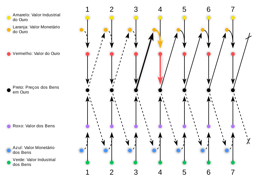
**7**. 🖍️ Let’s illustrate this for gold!
This diagram¹ depicts how gold transforms into money over time², rooted in its industrial (🟨) and monetary (🟧) values.
→ 1: Adapted from Figure 38, p. 274, of *Man, Economy and State* by Murray Rothbard.
→ 2: Time in the diagram reflects the sequence of events. The gap between 1-2 may differ from 2-3, but I’ll simplify it as Day Ⅰ, Ⅱ, Ⅲ, etc.
**8**. During Days Ⅰ-Ⅱ-Ⅲ, barter prevails¹: gold holds industrial value (🟨), such as in jewelry, setting prices for goods in gold (⬛) alongside the industrial value of those goods (🟩).
→ 1: The dashed lines between Days Ⅰ-Ⅱ-Ⅲ suggest "almost nothing," yet hint at the embryonic monetary value of gold (🟧). Some producers mine it with future trading in mind, initiating a monetary valuation even without direct exchanges.
**9**. On Day Ⅳ, someone trades for gold intending to resell it later! This marks the emergence of monetary value (🟧) in an exchange, after which both it and goods’ prices in gold (⬛) depend on past purchasing power, establishing temporal regression.
**10**. From Day Ⅴ onward, gold becomes a medium of exchange and, over time, gains enough widespread acceptance to be called money. This streamlines transactions, simplifies the price matrix¹, and boosts economic integration.
→ 1: (check **10.A.1-15** for more info, at the end).

#### Part 3.1 - The Bitcoin in Eternal Barter

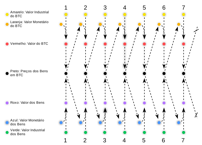
**11**. 💸 What if Bitcoin tried to become money in a world without currency, relying solely on barter?
In this scenario, no medium of exchange has ever emerged. Let’s explore how Bitcoin would fare!
**12**. In a barter system, Bitcoin needs industrial value (🟨) to take off. Unlike gold with its jewelry use, it lacks a common practical application. Could technological curiosity¹ give it value?
→ 1: E.g., miners experimenting with the system out of curiosity, though without broad demand.
**13**. Across Days Ⅰ-Ⅶ, Bitcoin’s industrial value (🟨) remains nearly zero. Without a practical purpose, demand would be scant—perhaps a "Bitcoin religious sect" might collect it for arbitrary reasons. But that’s a long shot!
**14**. For miners to trade bitcoins, they’d need buyers with genuine interest. This would only work in a rare Bitcoin-obsessed village—an unlikely prospect in a barter world.
**15**. Lacking significant industrial value, Bitcoin fails to develop monetary value (🟧) or purchasing power (⬛). It would linger as a "cryptographic toy," with slim chances of becoming a medium of exchange.
**16**. ♾️ In an eternal barter scenario, every trade is an isolated struggle, and Bitcoin would take forever to become money. Even gold would face challenges—it wasn’t humanity’s first medium (e.g., shells, salt). Bitcoin? Virtually impossible!

#### Part 3.2 - 🌱 Bitcoin Today

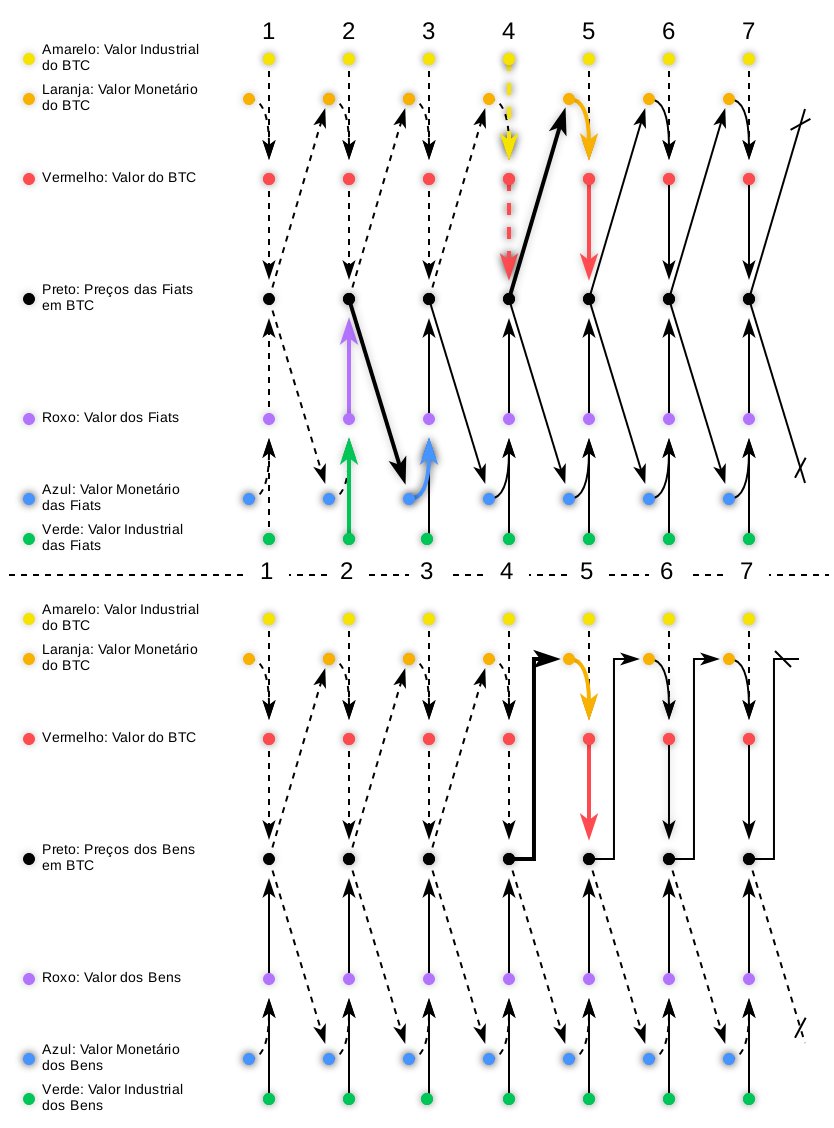
**17**. 🌍 Now, let’s look at Bitcoin today! Unlike the eternal barter scenario, we live in a world with fiat currencies (dollar, euro). How does Bitcoin become a medium of exchange here?
**18**. In the past, Day Ⅰ: the world relies on barter¹. Day Ⅱ: fiat emerges with industrial value (🟩), like paying taxes or avoiding penalties. Day Ⅲ²: fiat gains monetary value (🟦) and becomes money.
→ 1: We assume Bitcoin always existed, discovered in 2009 rather than invented, present since this hypothetical barter.
→ 2: Simplification: you can swap "fiat" for "gold" or assume gold’s history is omitted before Day Ⅱ.
**19**. Day Ⅳ: Bitcoin appears, carrying the same minimal industrial uses as in eternal barter. Yet, fiat now dominates: a pre-existing currency exists, the price matrix is established, and the economy is integrated.
**20**. The first miners understood money and envisioned future bitcoin trades.
🍞 To buy bread, they didn’t need a baker accepting bitcoins, just someone with dollars willing to trade. They sidestepped the double coincidence of wants!
**21**. They also recognized dollar censorship and saw the protocol’s potential: the energy costs ensuring Bitcoin’s immutability thrived in an integrated economy—a feat impossible in eternal barter!
**22**. 🌱 This context let Bitcoin skip the eternity needed for monetary speculation to emerge. It began in Bitcoin’s (factual) early days: on the 9th day, Satoshi traded bitcoins, donating some to Hal Finney.
**23**. ↱ Between transitions Ⅳ-Ⅴ, Bitcoin leverages the price matrix and economic integration. This is reflected in the lower section (Bitcoin vs. Goods) with a doubly orthogonal arrow¹.
→ 1: Here, the ↱ arrow applies to all goods in the economy, not just Bitcoin. All benefit from the simplified matrix, avoiding the double coincidence of wants with currency.
**24**. After 9 (factual) months, trades emerged on the New Liberty Standard Exchange: BTC×USD at 1000/1. We can assume some were buying bitcoins to resell, shown on Day Ⅴ with monetary value (🟧)¹.
→ 1: 🍕 Seven months later, "Pizza Day": pizzas bought via dollars (BTC×USD at 240/1). Two months after, MtGox (BTC×USD at 11/1). Six months later, Silk Road (BTC×USD at 1/1).
**25**. From Day Ⅴ, Bitcoin follows a temporal progression of monetary value (🟧), typical of a medium of exchange. Its price in current currency not only fluctuated but also soared over time!
**26**. Today, Bitcoin holds purchasing power, evident in its dollar price.
🤔 But is it evolving to enable direct exchanges with other goods, independent of the dollar’s economic integration and price matrix?

### Part 4 - Final Notes

**27**. This calls for a separate thread!
Thanks to everyone for following along!
A special thanks to my friend [@PedroSoyer_](https://x.com/PedroSoyer_) for his invaluable critiques and discussions!

### Part 5 - Sub-thread/Appendix: Price Matrix

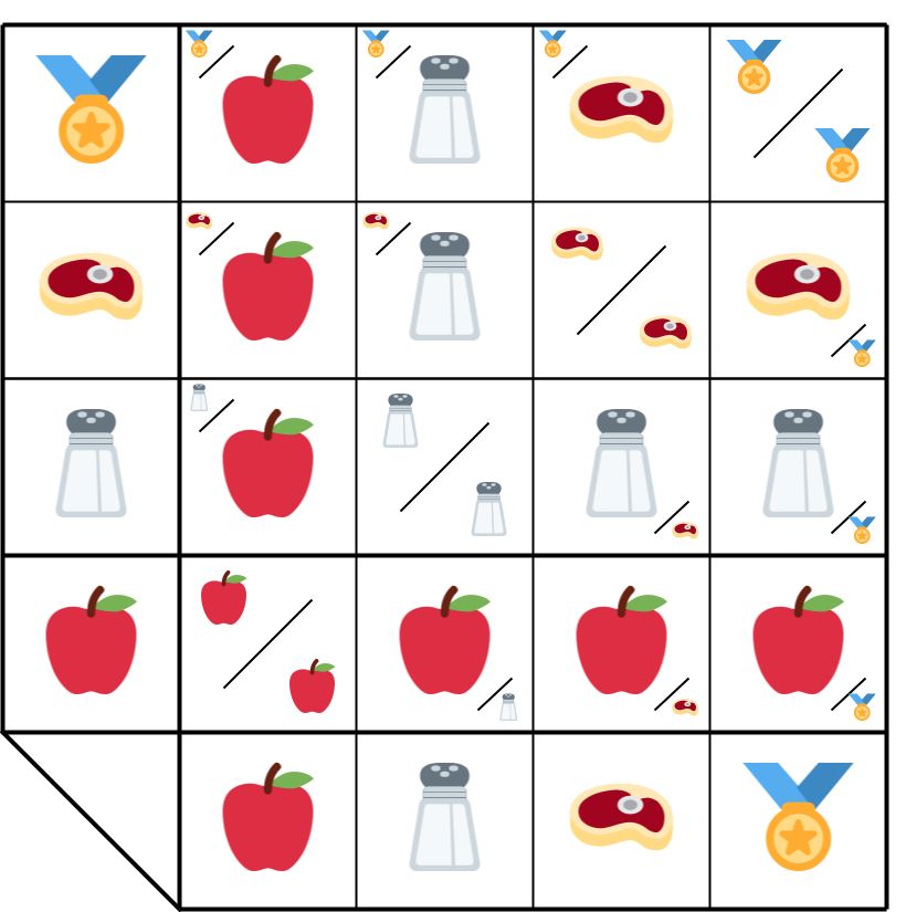
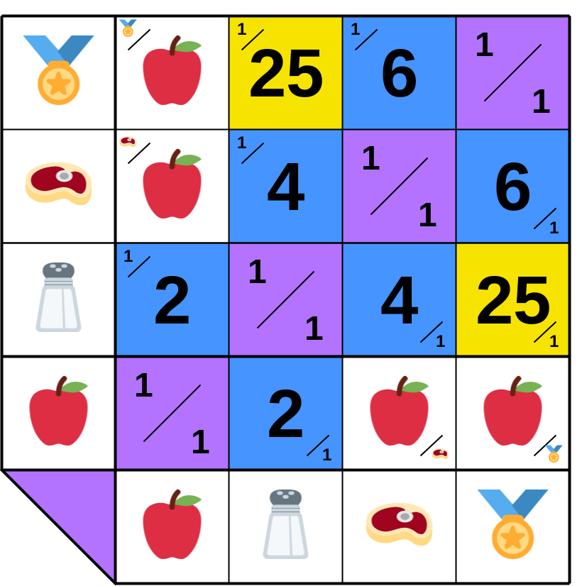
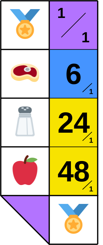
**10.A.1**.
→ 1: ▦ To grasp the price matrix, picture a world with 4 products (🍎🧂🥩🏅) and 4 people (𝔸-𝔹-ℂ-𝔻). Each inhabits an isolated island but can engage in chained trades (𝔸 ↔ 𝔹 ↔ ℂ ↔ 𝔻).

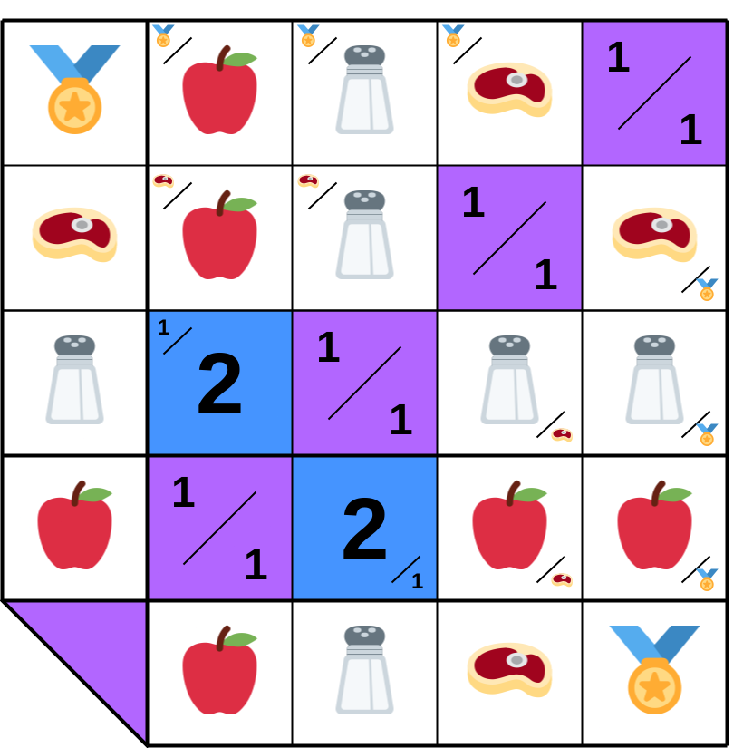
**10.A.2**. 𝔸 trades 2 units of 🍎 for 1 of 🧂 with 𝔹. In cell (🍎×🧂), the ratio is 2/1, and in (🧂×🍎), it’s 1/2.

**10.A.3**. Similarly, 𝔹 trades 4🧂 for 1🥩 with ℂ, who trades 6🥩 for 1🏅 with 𝔻. This builds a matrix of ratios, even in barter, where each cell (X×Y) represents a trade proportion between products (row×column).

**10.A.4**. 𝔸 can only trade with 𝔹 (𝔸 ↔ 𝔹). But what if 𝔸 wants 1🏅? Is it feasible? How many 🍎 must 𝔸 produce and save?
**10.A.5**. 𝔸 can estimate the ratio (🍎×🏅) ≈ ratio (🍎×🧂) × ratio (🧂×🥩) × ratio (🥩×🏅) = 2 × 4 × 6 = 48. Yet, this overlooks trade costs. The actual ratio emerges only with the trade.

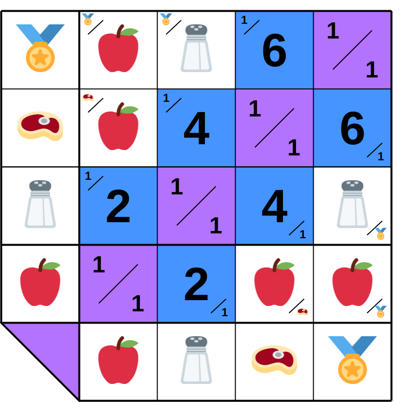
**10.A.6**. One option is for 𝔸 to ask 𝔹 to sell 1🏅. But doesn’t that recreate the same issue? 𝔹 can’t buy 🏅 directly (𝔸 ↔ 𝔹 ↔ ℂ). And since 𝔹 produces only 🧂, how many would be needed?
**10.A.7**. 𝔹 can predict the ratio (🧂×🏅) ≈ ratio (🧂×🥩) × ratio (🥩×🏅) = 4 × 6 = 24. However, this remains a forecast, not the true ratio.

**10.A.8**. 𝔹 can ask ℂ to sell 1🏅! ℂ buys 1🏅 from 𝔻 for 6🥩 and resells it for 6🥩 + 1🧂, all in 🧂, i.e., 6 × ratio (🧂×🥩) + 1 = 6 × 4 + 1 = 25. A new ratio enters the matrix!

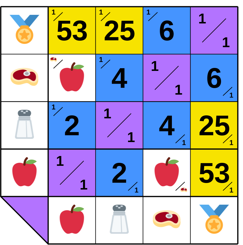
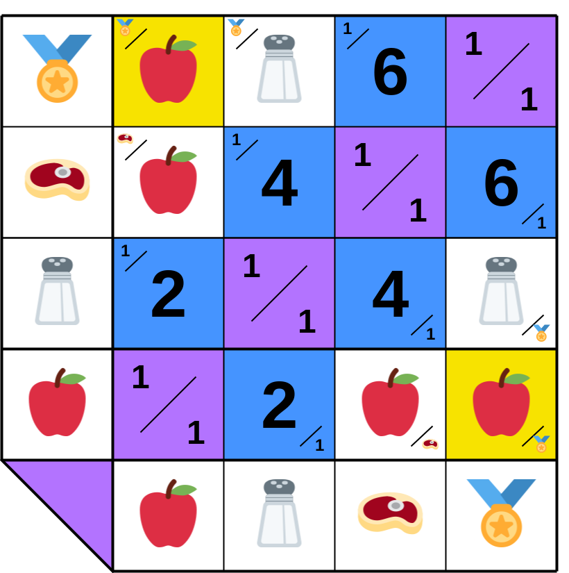
**10.A.9**. 𝔹 buys 1🏅 from ℂ for 25🧂 and resells it for 25🧂 + 3🍎, all in 🍎, i.e., 25 × ratio (🍎×🧂) + 3 = 25 × 2 + 3 = 53. 𝔸’s desired trade can now proceed with a set ratio!
**10.A.10**. Thus, a chain of trades fills ratios between goods (🍎×🏅), even without direct exchanges. However, trade costs can render the initial prediction of (🍎×🏅) = 48/1 unrealistic.
**10.A.11**. 𝔸 got lucky, as 𝔹 agreed to trade 53🍎 for 25🧂, and as the trades 𝔹 ↔ ℂ and ℂ ↔ 𝔻 fell into place. But this isn’t guaranteed! 𝔸 relied on a coincidence of interests with 𝔹, ℂ, and 𝔻. Longer chains amplify uncertainties.

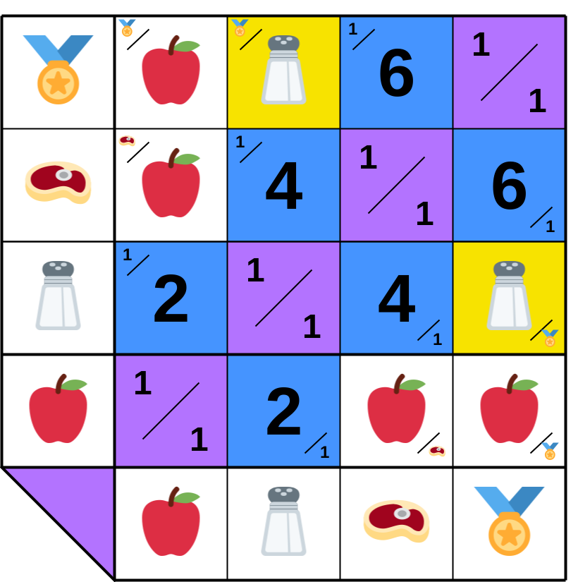
**10.A.12**.
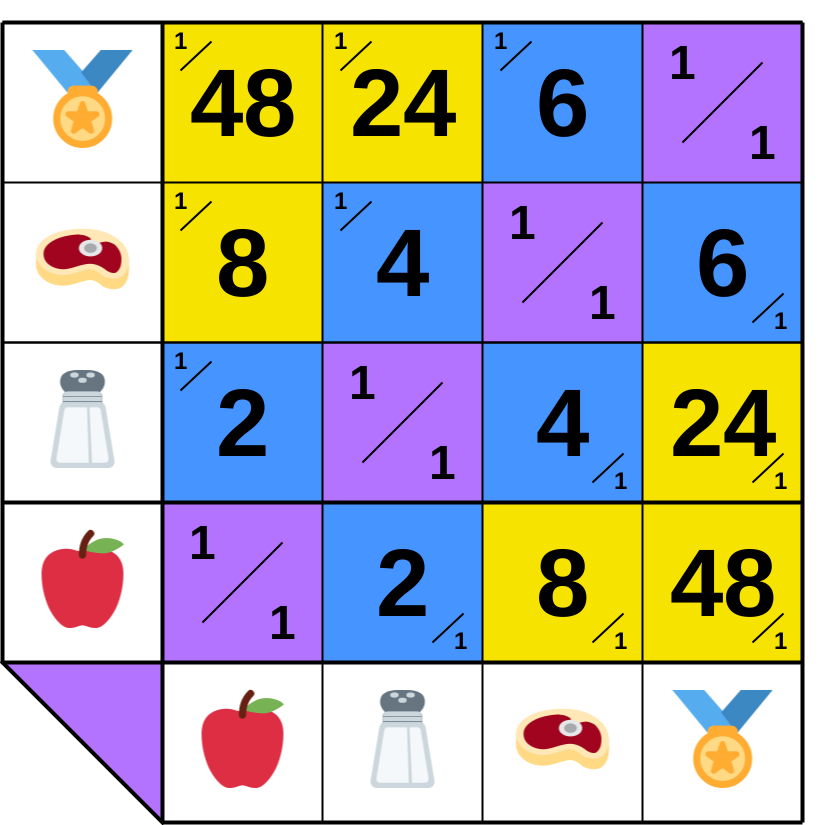
But if trades incur no costs and 🏅 becomes money, ▦ the matrix simplifies,

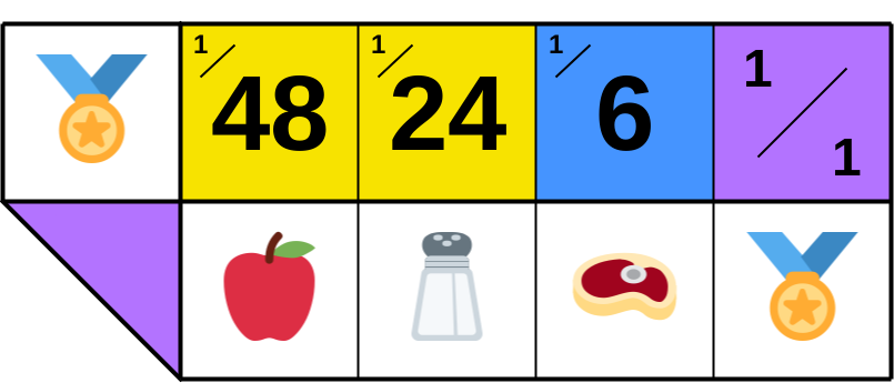
▭ with ratios denominated solely in 🏅

and by symmetry, ▯ all products also denominate it.

Planning then centers on the currency, enhancing economic integration.

**10.A.13**. 🤔 So, what’s the point of this "economic integration"?
It enables easier planning, specialization, and labor division, boosting productivity and wealth for all involved.
**10.A.14**. 🤔 Even with currency, don’t multiple trades still occur before buying something like a 🔭?
Yes, but 𝔸 doesn’t need to orchestrate them. Economic integration lets this emerge rationally from market participants.

[Youtube: "What if there were no prices?"](https://www.youtube.com/watch?v=zkPGfTEZ_r4)

**10.A.15**. Notably, money eliminates the cost of the double coincidence of wants—the "luck" 𝔸 needed for others to accept the trade chain. With a currency everyone wants to earn and spend, this cost vanishes.