# 通訊實驗matched filter結報
###### tags: `通訊` `matlab`
###### 撰寫時間 : 2022/05/13

## 實驗目的
- 接收端利用匹配濾波器，配合適當取樣時間來解調傳送端傳送的的兩波形所代表的二位元信號。
- 如何模擬實現匹配濾波器。

## matched filter 實驗原理
1. 首先binary sequence $b_k \in \{0,1\}$，會進行訊號調變(modulation)，這裡使用pulse amplitude modulation(PAM)，首先每個bit通過symbol mapper，將每個bit映射到一個數值，分為以下兩種
$$
\begin{align*}
&\text{In antipodal signaling,}& a_k
\begin{cases}
1, &b_k = 1\\
-1, &b_k = 0
\end{cases}
\Rightarrow a_k = 2b_k-1\\
&\text{In on-off signaling,}& a_k
\begin{cases}
1, &b_k = 1\\
0, &b_k = 0
\end{cases} \Rightarrow a_k = b_k
\end{align*}
$$
2. 接下來通過一個pulse shaping filter $g'(t)$，一般$g'(t)$使用方波，調變後的訊號$s(t)$就是$a_kg'(t - kT)$，$a_k$就是代表這個波型的振幅。
3. 通過一個channel，一般假設是AWGN channel，因此接收端接收到的訊號就是$r(t) = s(t) + w(t)$。
4. 接收端通過一個filter，為了得到極大化SNR值，這個filter會根據輸入訊號$s(t)$的波型，設計一個match $s(t)$的波型，設計準則為將輸入訊號先做反轉再做延遲$g(t) = s(\underbrace{-}_{\text{inverse} }(t \underbrace{- T}_{\text{delay T} }) )$。
5. 取樣一段時間後才會輸出訊號，當取樣時間$t = T$，此時matched filter等於correlator，而若$g(t)$又是方波，matched filter等效上積分器，而從電子學可知積分器可以過濾高頻雜訊。
6. 最後是一個判斷機制，判斷這個數值是0和1，需要設計一個threshold $\gamma$，極小化位元錯誤率$P_e$。

- **最大化$Y(T)$(當$Y(t)$取樣時間$t = T$)的SNR，使對抗雜訊的能力增加**<br>
首先先正規化received filter的限制為$\int^T_0 |g(t)|^2 dt = T$。
$$
\begin{align*}
Y &= g(t) * r(t)\\
&= \int^T_0 g(T - \tau) [s(\tau) + w(\tau)] d\tau\\
&= \underbrace{\int^T_0 g(T - \tau)s(\tau) d\tau}_{\text{desird part(signal)}} + \underbrace{\int^T_0 g(T - \tau) w(\tau) d\tau}_{\text{noise part}}\\
&\text{goal :} \max \{\text{SNR}\} = \max \{ \frac{ P_{\text{signal}} }{ P_{\text{noise}} } \}
\end{align*}
$$
要求出noise的power$P_{\text{noise}}$就是取其變異數(二階動差 - 一階動差平方)，代表是AC的power(總功率的power - DC的power)。
$$
\begin{align*}
\text{Let } N &= \int^T_0 g(T - \tau)w(\tau)d\tau\\
\text{mean of } N : E[N] &= \int^T_0 g(T - \tau) \underbrace{E[w(\tau)]}_{ = 0} d\tau = 0\\
\text{variance of } N : \mathrm{Var}\{N\} &= E[N^2] - ( \underbrace{E[N]}_{=0} )^2\\
&= R_N(0) = \mathscr{F}^{-1}\{S_N(f)\}\\
&= \int^\infty_{-\infty} S_N(f) e^{+j2\pi f \cdot 0}df\\
&= \int^\infty_{-\infty} S_N(f) df\\
&= \int^\infty_{-\infty} |G(f)|^2S_W(f) df &\because \text{WSS process pass LTI system }G(f)\\
&= \frac{N_0}{2}\int^\infty_{-\infty} |G(f)|^2 df\\
&= \frac{N_0}{2}\int^\infty_{-\infty} |g(t)|^2 dt &\because \text{Parseval's theorem}\\
&= \frac{N_0}{2}\int^T_0 |g(t)|^2 dt &\because \text{constraint term} \int^T_0 |g(t)|^2 dt = T\\
&= \frac{N_0}{2}\int^T_0 |g(T - t)|^2 dt &\because \text{change of variables}
\end{align*}
$$
因此SNR可以改寫為
$$
\text{SNR}_Y = \frac{ P_{\text{signal}} }{ P_{\text{noise}} } = \frac{ [\int^T_0 g(T - \tau) s(\tau) d\tau]^2 }{\frac{N_0}{2}\int^T_0 |g(T - t)|^2 dt}
$$
由於底下該項是常數，因此使用柯西不等式，可以求出SNR所能到達最大值為
$$
\begin{align*}
\text{SNR}_Y &= \frac{ [\int^T_0 g(T - \tau) s(\tau) d\tau]^2 }{\frac{N_0}{2}\int^T_0 |g(T - t)|^2 dt}
\leq \frac{ [\int^T_0 |g(T - \tau)|^2d\tau]\cdot [ \int^T_0 |s(\tau)|^2 d\tau] }{\frac{N_0}{2}\int^T_0 |g(T - t)|^2 dt} = \underbrace{\frac{2}{N_0} \int^T_0 |s(\tau)|^2d\tau}_{\text{only depends on energy of }s(t) }
\end{align*}
$$
等號成立的條件為兩向量平行，即為$g(T - \tau) = cs(\tau)$或是$g(\tau) = cs(T - \tau) = cs(-(\tau - T))$，物理意義就是將輸入訊號先做反轉再做延遲，此received filter設計就是matched filter。

## lab1
問題 : duration設定為4 symbol periods， 畫出在$\frac{E_b}{N_0} = 10 \;\rm dB$與$\frac{E_b}{N_0} = 3 \;\rm dB$的transmitted waveform和received waveform並比較差異。

|$\frac{E_b}{N_0} = 10 \;\rm dB$|$\frac{E_b}{N_0} = 3 \;\rm dB$|
|:-:|:-:|
|||

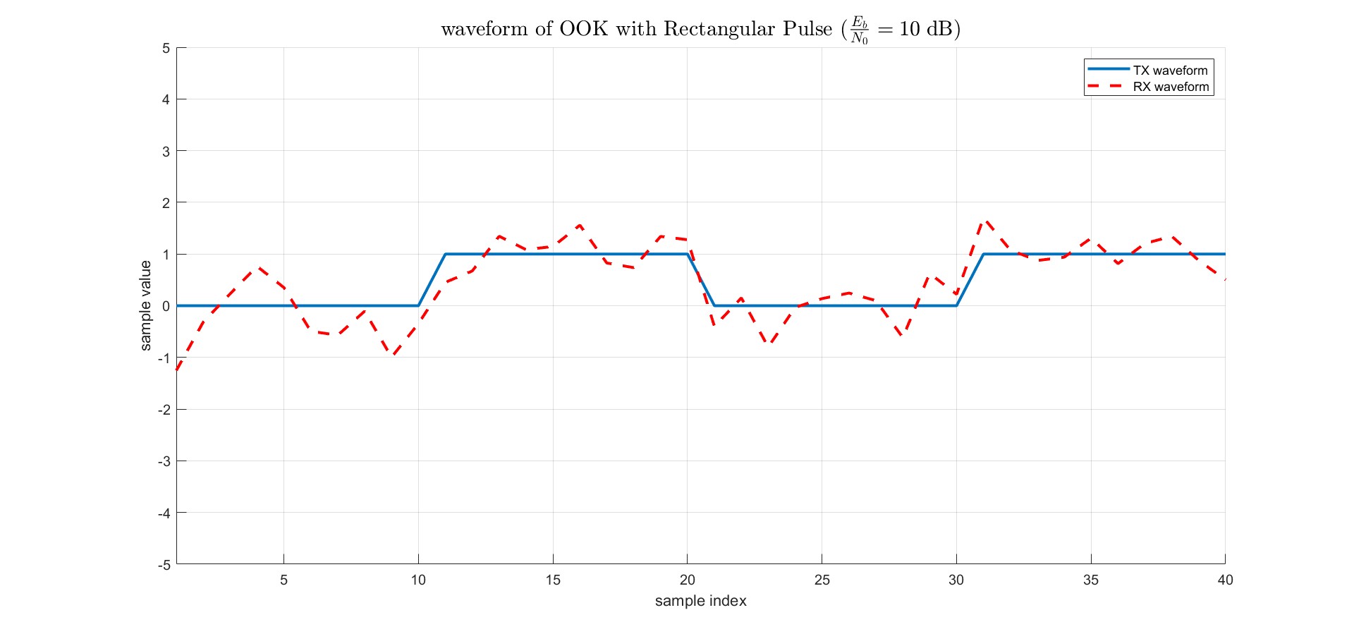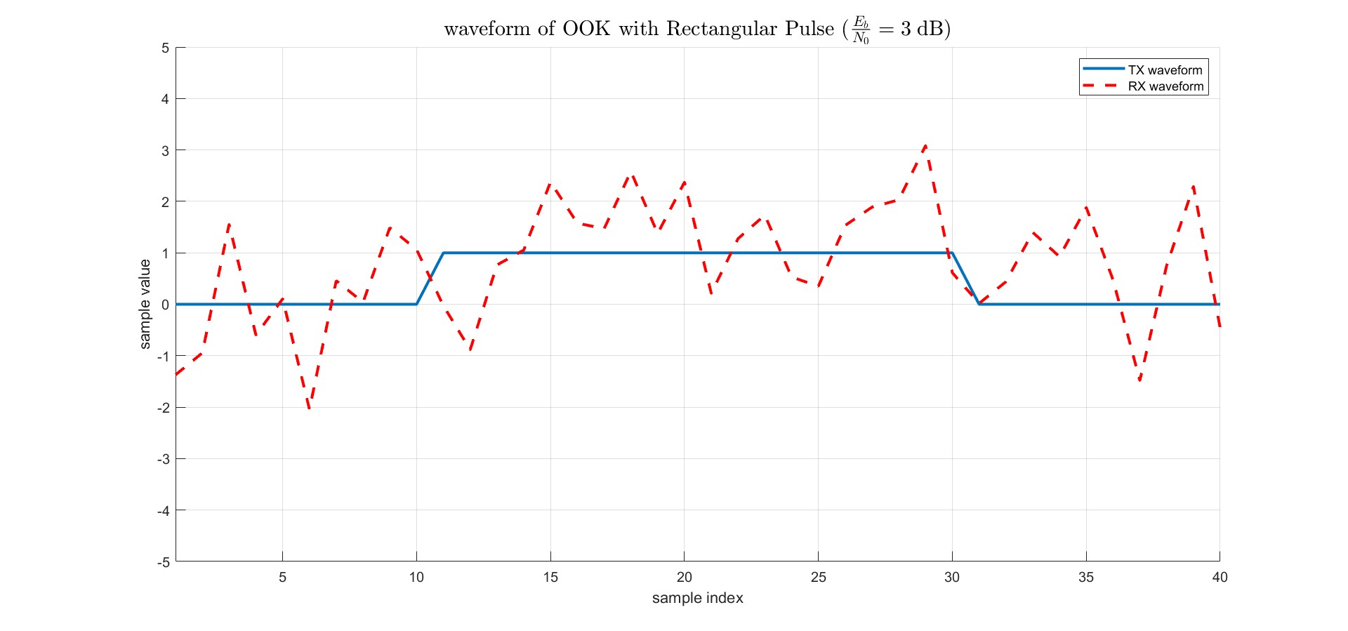定義信噪比$\text{SNR}_o \triangleq \frac{ P_{\text{signal}} }{ P_{\text{noise}} } \triangleq \frac{E_b}{N_0}$ ，其中$N_0$代表高斯雜訊的一個定值($S_w(f) \triangleq \frac{N_0}{2}$)、$E_b$代表on-off keying每個bit的平均能量$E_b = \frac{1}{2}A^2T + \frac{1}{2} \cdot 0 = \frac{A^2T}{2}$，因此降低SNR，$N_0$保持一致，等同降低降低每個bit傳送時的平均能量，由於$P_e = \mathrm{Q}(\sqrt{\text{SNR}})$，因此BER會變差。

而範例程式這邊與我上述直覺**理解不同點**是在維持$E_b$下，調動noise的power $\sigma^2$，降低SNR，會讓$\sigma^2$變大，因此接收端(RX)訊號右圖會比左圖變化幅度還大。

## lab2-1
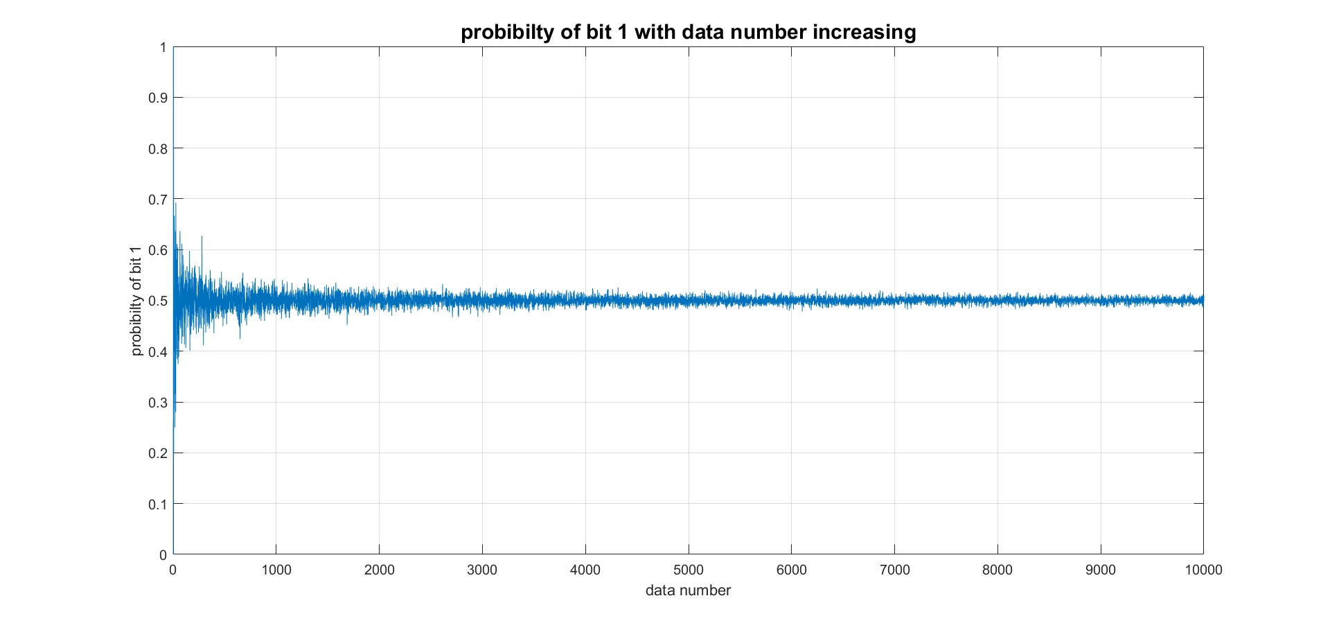
問題 : 解釋程式`Data_bit = (rand(1, data_number) > 0.5 )`為何可產生random bits?bit 0 和bit 1，其發生機率理論上應為何?實際於模擬是否符合理論預測？

指令`rand(M,N)`代表返回一個$M \times N$的矩陣，每個element的值是取區間0到1的均勻分布$ U \sim (0, 1)$並使用logic判斷式判斷是否大於0.5，若符合回傳1，反之回傳0，回傳的data type是`logic`。

由於是均勻分布，0到0.5的區間機率是$\frac{1}{2}$，判定為logic 0；0.5到1的區間機率是$\frac{1}{2}$，判定為logic 1，實際模擬如下圖
<br>
藉由做很多次的隨機試驗，可以得到relative frequency $f_n(A) = \frac{N_n(A)}{n}$，當試驗次數越多，會趨於機率，記為$\lim_{n \to \infty} f_n(A) = P(A)$，由上圖可知data number越多，機率會趨於$\frac{1}{2}$。

## lab2-2
問題 :

data_number = 10^5; % # of bits
Fs = 10; % sampling frequency (used to generate received samples)
Data_bit = (rand(1,data_number) > 0.5 ); % random bits
p1 = ones(1,Fs); % discrete‐time rectangular pulse that represents one symbol
Data_pulse_array = (p1') * Data_bit;
Data_pulse = reshape(Data_pulse_array,1,length(p1)*data_number);

其中`Data_pulse = reshape(Data_pulse_array, 1, length(p1)*data_number)`代表意義。

`Data_bit`為由機率各半($\frac{1}{2}$)的logic 0和1形成$1 \times 10^5$的矩陣，`Data_pulse_array`為將`Data_bit`的值拷貝成$10 \times 10^5$的矩陣，此時data type是`double`，最後`reshape`將$10 \times 10^5$的矩陣，以column為順序，轉換為`(1,length(p1)*data_number)`的矩陣，代表意義是每10個單位傳送一個symbol。

## lab3
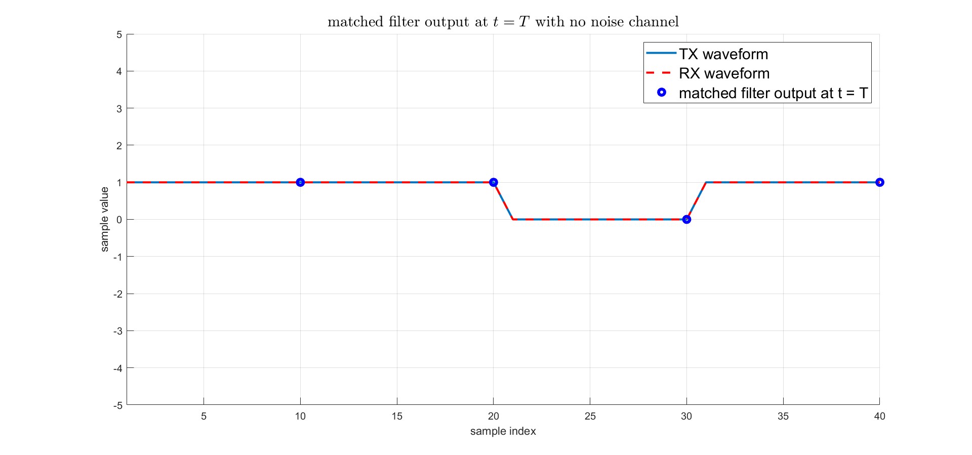
問題 : 沒有雜訊下，matched filter output $y(T)$理論值與模擬值為何?

Data_receive = Data_pulse; % received samples
D_filtered = conv(Data_receive,p1); % MF output
D_demapping = D_filtered(10:10:end) / 10; % sampling at symbol rate

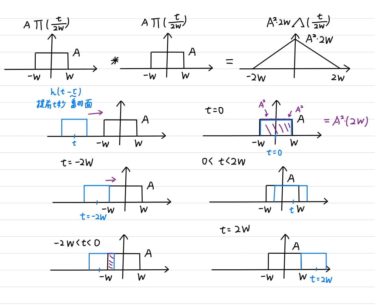
首先計算兩方波做convolution，如下圖所示
<br>
兩個方波做convolution等於一個三角波，數學式記為
$$
[A \cdot \Pi(\frac{t}{2W})] * [A \cdot \Pi(\frac{t}{2W})] = A^2 \cdot 2W \cdot \Lambda(\frac{t}{2W})
$$
由於本題假設沒有雜訊，因此傳送端訊號等於接收端訊號，接下來與matched filter做convolution計算為根據上述知識，使用$A = 1, 2W= 10$，可計算結果，使用matlab模擬驗證，假設傳送bit為`1101`，matched filter output $y(t)$如下<br>
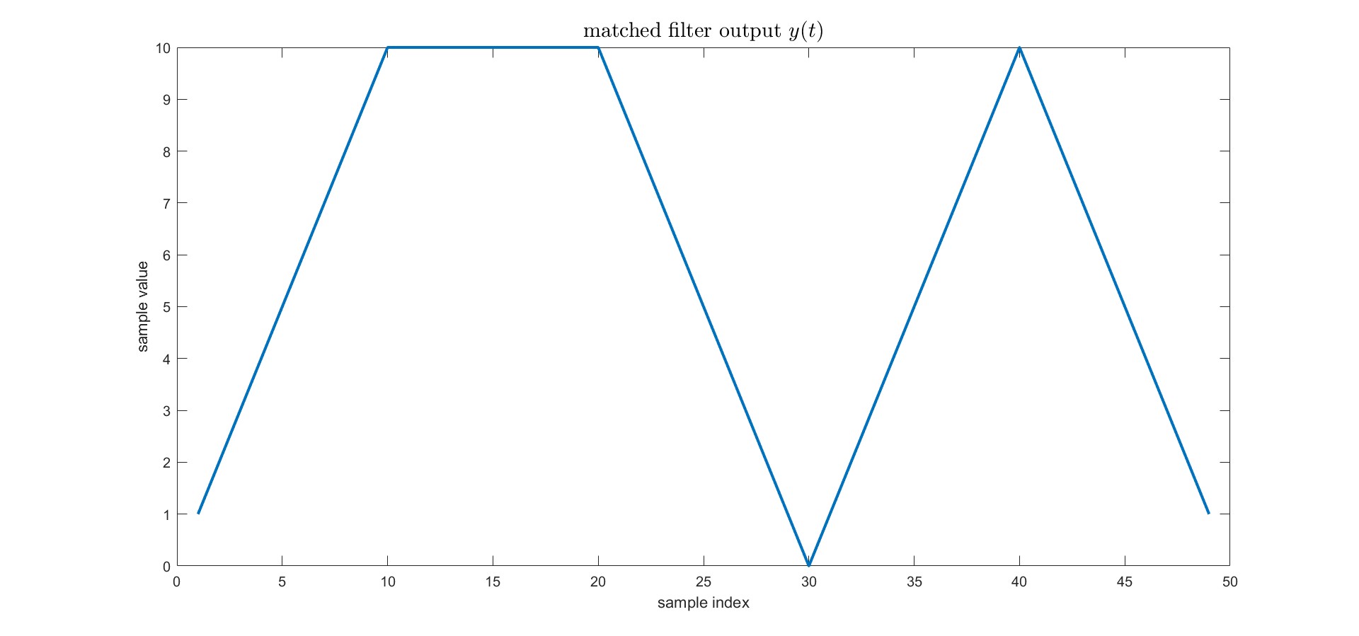<br>
取$y(t)$中$t = T$時刻的時間，即上圖中simple index在10、20、30、40下的值，由於大小是$A^2 \cdot 2W$，因此需要除以一個scaling $A \cdot 2W$轉為原本波型的大小$A$，本題就是$A \cdot 2W = 1 \cdot 2 \cdot 5 = 10$，最後繪製如下圖，藍點代表$y(T)$是時間在10、20、30、40下的數值除以一個10的scaling。

## lab4
問題 : 解釋`D_demapping=D_filtered(10:10:end)/10`。

同lab3問題，取matched filter在$t = T$下的輸出，並除上一個$A \cdot 2W = 1 \cdot 2 \cdot 5 = 10$的scaling。

## lab5
問題 : 解釋`sgma = sqrt( 0.5/EbN0/2*10 )`。

如lab1觀念，定義信噪比$\text{SNR}_o \triangleq \frac{ P_{\text{signal}} }{ P_{\text{noise}} } \triangleq \frac{E_b}{N_0}$ ，其中$N_0$代表高斯雜訊的一個定值($S_w(f) \triangleq \frac{N_0}{2}$)、$E_b$代表on-off keying每個bit的平均能量$E_b = \frac{1}{2}A^2T + \frac{1}{2} \cdot 0 = \frac{A^2T}{2}$，由於本題條件$A = 1, T = 1$，因此$E_b = \frac{1}{2}$，另外假設取樣頻率$T_s = 10$，每個sample point的noise power為$\sigma_s^2$，計算$\sigma_s^2$值如下
$$
\begin{align*}
\text{Let } N &= \int^T_0 g(T - \tau)w(\tau)d\tau\\
\text{mean of } N : E[N] &= \int^T_0 g(T - \tau) \underbrace{E[w(\tau)]}_{ = 0} d\tau = 0\\
\sigma_s^2 &= \frac{1}{T_s} \cdot \sigma^2\\
&= \frac{1}{T_s} \cdot (E[N \cdot N] - E[N]^2)\\
&= \frac{1}{T_s} \cdot \int^T_0 \int^T_0 E[w(t) \cdot w(\tau)]dtd\tau &\because E[N] = 0\\
&= \frac{1}{T_s} \cdot \int^T_0 \int^T_0 R_w(t - \tau) dtd\tau &\because \text{noise is SSS} \in \text{WSS}\\
&= \frac{1}{T_s} \cdot \int^T_0 \int^T_0 \frac{N_0}{2} \delta(t - \tau) dtd\tau\\
&= \frac{1}{T_s} \cdot \frac{N_0}{2}\\
\Rightarrow & N_0 = 2 \cdot T_s \cdot \sigma_s^2
\end{align*}
$$

SNR可改寫為
$$
\text{SNR}_o \triangleq \frac{ P_{\text{signal}} }{ P_{\text{noise}} } \triangleq \frac{E_b}{N_0} =\frac{ \frac{A^2T}{2} }{ 2 \cdot T_s \cdot \sigma_s^2 } = \frac{ \frac{1}{2} }{ 2 \cdot 10 \cdot \sigma_s^2 }
$$

## lab6
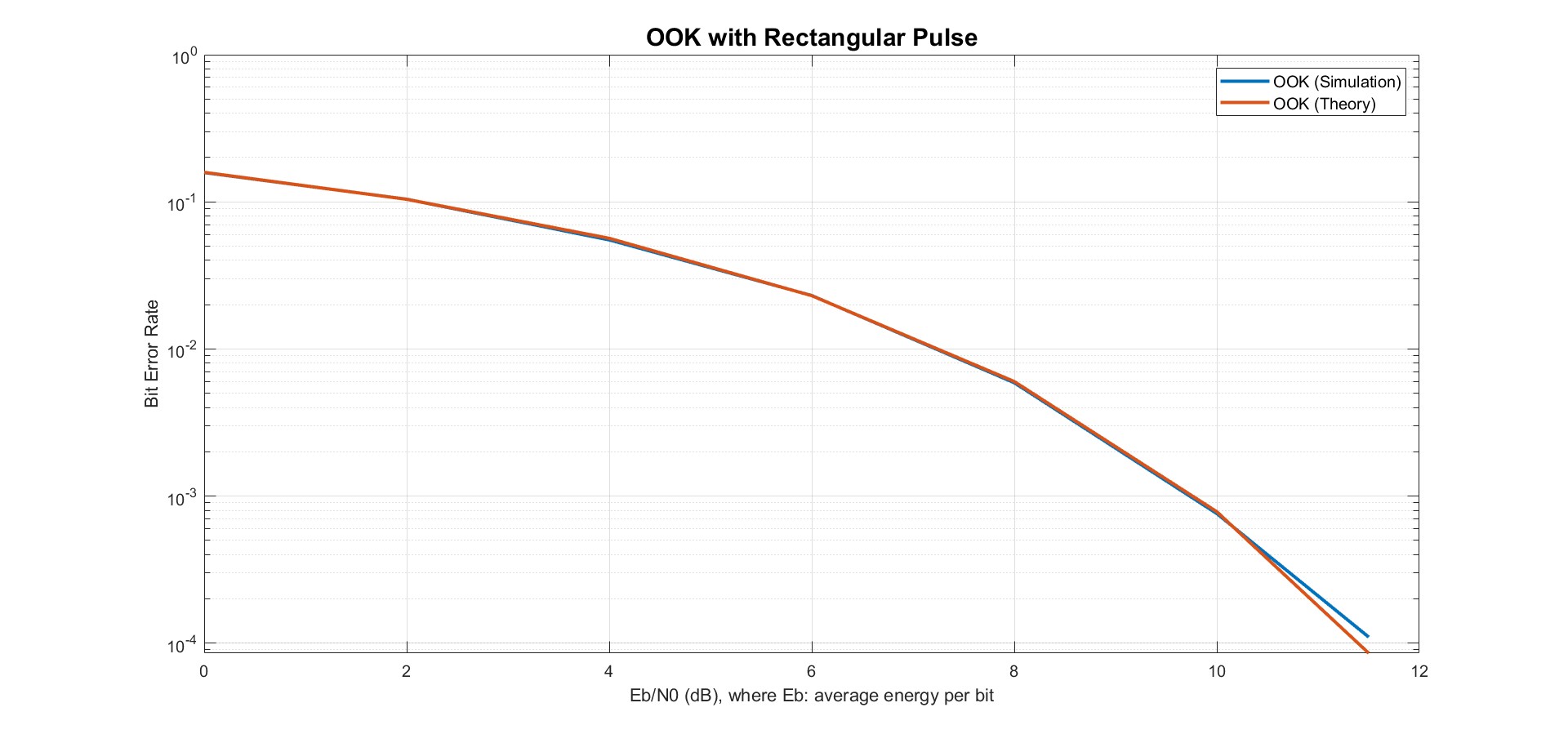
問題 : 畫出OOK中BER對SNR理論值與實際值做圖。

在機率equally likely $p = q = \frac{1}{2}$條件下，OOK的bit error rate(BER)理論值計算為
$$
\begin{align*}
P_e &= \int^\infty_{\frac{AT}{2\sigma}} \frac{1}{\sqrt{2\pi}} e^{-\frac{y^2}{2}}dy\\
&= \mathrm{Q}(\frac{AT}{2\sigma})\\
&= \mathrm{Q}(\frac{AT}{2 \sqrt{\frac{N_0 T}{2}}})\\
&= \mathrm{Q}(\sqrt{\frac{A^2T}{2} \cdot \frac{1}{N_0}})\\
&= \mathrm{Q}(\sqrt{\frac{E_b}{N_0}})
\end{align*}
$$
與實際用matlab模擬值

 D_demap_N = (D_demapping > 0.5); % >0.5: 1; <=0.5: 0
 % BER computation
 Error_num = sum(xor(D_demap_N,Data_bit)); % same -> 0; diff -> 1
 BER = Error_num/data_number;

繪圖如下<br>
<br>
由上圖可知理論值計算與matlab模擬值之間誤差非常小。

## lab7
問題 : 在$\frac{E_b}{N_0} = 10 \;\rm dB$與$\frac{E_b}{N_0} = 3 \;\rm dB$的情況下，畫出matched filter output $y(T)$的conditional pdf $f(y(T)| \text{bit 0 sent})$與$f(y(T)| \text{bit 1 sent})$的理論值與模擬值。

index_0 = 1;
for i = 1:data_number
    if Data_bit(i) == 0 % TX == 0
        D_demapping_0(index_0) = D_demapping(i);
        index_0 = index_0 + 1;
    end
end

如果一開始傳送訊號是`0`，提取輸出訊號$y(T)$並存入另一個自定義的array，代表**選取指定事前機率下的輸出數據**。

histogram(D_demapping_0, 'FaceColor', '#0072BD','Normalization','pdf');

下指令`histogram(X,'Normalization','pdf')`畫各個數值區間內的統計數量，[後面那2個參數](https://www.mathworks.com/help/matlab/ref/matlab.graphics.chart.primitive.histogram-properties.html)是取數據`X`的probability density function。

plot(xaxis,normpdf(xaxis,0,sgma / sqrt(10)), 'LineWidth',3);

理論值計算下指令`normpdf`，代表使用常態(高斯)分布$N \sim (\mu, \sigma^2)$，其中mean $\mu$是0，而standard deviation(標準差) $\sigma$是需要乘以$\frac{1}{\sqrt{10}}$的scaling，原因是根據[lab3](#lab3)觀念，經過convolution後的訊號要除以$10$的scaling才是最終的$y(T)$，$y(T)$其中也包括雜訊$N \sim (0, \sigma^2)$，因此$\sigma^2 \rightarrow \frac{\sigma^2}{10} \Rightarrow \sigma \rightarrow \frac{\sigma}{\sqrt{10}}$。

分別就不同SNR$\frac{E_b}{N_0}$下畫出conditional pdf$f(y(T)| \text{bit 0 sent})$與$f(y(T)| \text{bit 1 sent})$的理論值與模擬值。
|$\frac{E_b}{N_0} = 10 \;\rm dB$|$\frac{E_b}{N_0} = 3 \;\rm dB$|
|:-:|:-:|
|||

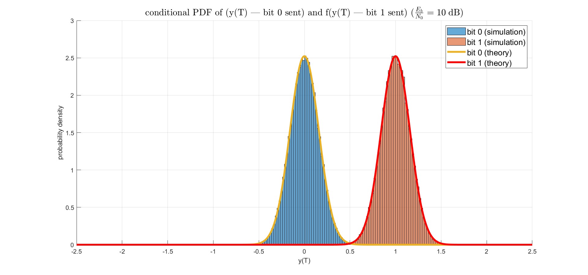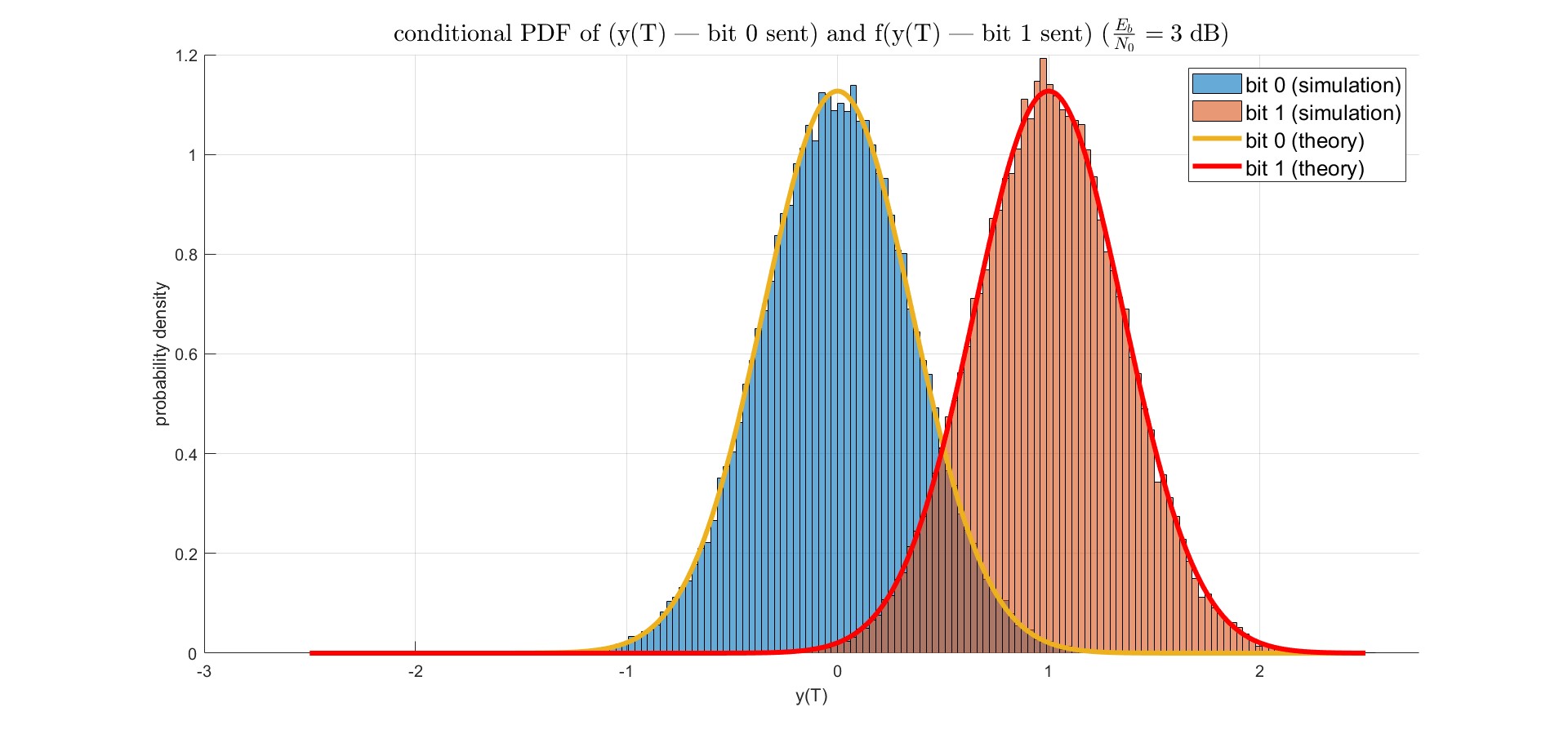降低SNR，在維持$E_b$的條件下，調動noise的power $\sigma^2$，會讓$\sigma^2$變大，因此右圖的PDF會比左圖的PDF還矮胖。

## 程式
- lab1

% matched filter
% ‐ on‐off keying (OOK) using rectangular pulse (T=1)
% That is, when OFF, assuming A=0, thus E1 = 0
% when ON: assuming A=1, thus E2 = 1
% The "average bit energy" (Eb) = (E1+E2)/2 = 1/2
%
clear,clc,close all;
%% parameters
data_number = 4; % # of bits
Fs = 10; % sampling frequency (used to generate received samples)

%% transmitter
Data_bit = (rand(1,data_number) > 0.5 ); % random bits
p1 = ones(1,Fs); % discrete‐time rectangular pulse that represents one symbol
Data_pulse_array = (p1')*Data_bit;
Data_pulse = reshape(Data_pulse_array,1,length(p1)*data_number);

%% AWGN channel and receiver
% AWGN channel
EbN0dB = 10; % 3 10
[a, b] = size(Data_pulse);
EbN0 = 10^(EbN0dB/10); % EbN0 is now in linear scale
sgma = sqrt( 0.5/EbN0/2*10);
noise = normrnd(0, sgma, a, b);
Data_receive = Data_pulse + noise; % received samplesa

%% generate plots
figure;
xais = 1:40;
hold on;
plot(xais, Data_pulse, 'LineWidth',2);
plot(xais, Data_receive, '--r', 'LineWidth',2);
ylim([-5 5]);
xlim([1 40]);
xlabel('sample index');
ylabel('sample value');
legend('TX waveform', 'RX waveform');
grid on;
title('waveform of OOK with Rectangular Pulse ($\frac{R_b}{N_0} = 10 \;\rm dB$)','Interpreter','latex','FontSize',15);

- lab2

clear,clc,close all;

pro_1 = zeros(1, 20); % preallocate memory
for k = 1:10^4
    sum_1 = 0;
    data_number = k; % # of bits
    Data_bit = (rand(1,data_number) > 0.5 ); % random bits
    for i = 1:data_number
        if Data_bit(i) == 1
            sum_1 = sum_1 + 1;
        end
    end
    pro_1(k) = sum_1 ./ data_number;
end

xais = 1:10^4;
plot(xais, pro_1);
ylim([0, 1]);
xlabel('data number');
ylabel('probibilty of bit 1');
grid on;
title('probibilty of bit 1 with data number increasing','FontSize',15);

- lab3

% matched filter
% ‐ on‐off keying (OOK) using rectangular pulse (T=1)
% That is, when OFF, assuming A=0, thus E1 = 0
% when ON: assuming A=1, thus E2 = 1
% The "average bit energy" (Eb) = (E1+E2)/2 = 1/2
%
clear,clc,close all;
%% parameters
data_number = 4; % # of bits
EbN0dB_vec = [0:2:10 11.5]; % Eb/N0 in dB
Fs = 10; % sampling frequency (used to generate received samples)

%% transmitter
Data_bit = (rand(1,data_number) > 0.5 ); % random bits
p1 = ones(1,Fs); % discrete‐time rectangular pulse that represents one symbol
Data_pulse_array = (p1')*Data_bit;
Data_pulse = reshape(Data_pulse_array,1,length(p1)*data_number);

%% no AWGN channel and receiver
Data_receive = Data_pulse; % received samples
% receiver
D_filtered = conv(Data_receive,p1); % MF output
D_demapping = D_filtered(10:10:end) / 10; % sampling at symbol rate
% decsion based on D_demapping
D_demap_N = (D_demapping > 0.5); % >0.5: 1; <=0.5: 0

%% generate plots
figure;
xaxis = 1:40;
hold on;
plot(xaxis, Data_pulse, 'LineWidth',2);
plot(xaxis, Data_receive, '--r', 'LineWidth',2);

for i = 1:4
    scatter(10*i, D_demapping(i),'b', 'LineWidth',3);
end

ylim([-5 5]);
xlim([1 40]);
xlabel('sample index');
ylabel('sample value');
legend('TX waveform', 'RX waveform', 'matched filter output at t = T','FontSize',15);
grid on;
title('matched filter output at $t = T$ with no noise channel','Interpreter','latex','FontSize',15);
hold off;

% xaxis_49 = 1:49;
% plot(xaxis_49, D_filtered, 'LineWidth',2);
% xlabel('sample index');
% ylabel('sample value');
% title('matched filter output $y(t)$','Interpreter','latex','FontSize',15);

- lab6

% matched filter
% ‐ on‐off keying (OOK) using rectangular pulse (T=1)
% That is, when OFF, assuming A=0, thus E1 = 0
% when ON: assuming A=1, thus E2 = 1
% The "average bit energy" (Eb) = (E1+E2)/2 = 1/2
%
clear,clc,close all;
%% parameters
data_number = 10^5; % # of bits
EbN0dB_vec = [0:2:10 11.5]; % Eb/N0 in dB
Fs = 10; % sampling frequency (used to generate received samples)

%% transmitter
Data_bit = (rand(1,data_number) > 0.5 ); % random bits
p1 = ones(1,Fs); % discrete‐time rectangular pulse that represents one symbol
Data_pulse_array = (p1')*Data_bit;
Data_pulse = reshape(Data_pulse_array,1,length(p1)*data_number);

%% AWGN channel and receiver
BER = zeros(1, length(EbN0dB_vec)); % pre-allocate
BER_theory = zeros(1, length(EbN0dB_vec)); % pre-allocate
for kk=1:length(EbN0dB_vec)
    % AWGN channel
    [a, b] = size(Data_pulse);
    EbN0dB = EbN0dB_vec(kk);
    EbN0 = 10^(EbN0dB/10); % EbN0 is now in linear scale
    sgma = sqrt( 0.5/EbN0/2*10);
    noise = normrnd(0, sgma, a, b);
    Data_receive = Data_pulse + noise; % received samples
    % receiver
    D_filtered = conv(Data_receive,p1); % MF output
    D_demapping = D_filtered(10:10:end) / 10; % sampling at symbol rate
    % decsion based on D_demapping
    D_demap_N = (D_demapping > 0.5); % >0.5: 1; <=0.5: 0
    % BER computation
    Error_num = sum(xor(D_demap_N,Data_bit)); % same -> 0; diff -> 1
    BER(kk) = Error_num/data_number;
    % fprintf('EbN0 in dB is %g\n',EbN0dB);
    % fprintf('Bit error rate is %g\n',BER);
    BER_theory(kk) = qfunc(sqrt(EbN0));
end

%% generate plots
figure;
semilogy(EbN0dB_vec, BER, EbN0dB_vec, BER_theory, 'LineWidth',2);
xlabel('Eb/N0 (dB), where Eb: average energy per bit');
ylabel('Bit Error Rate');
legend('OOK (Simulation)', 'OOK (Theory)','FontSize',10);
grid on;
title('OOK with Rectangular Pulse','FontSize',15);

- lab7

% matched filter
% ‐ on‐off keying (OOK) using rectangular pulse (T=1)
% That is, when OFF, assuming A=0, thus E1 = 0
% when ON: assuming A=1, thus E2 = 1
% The "average bit energy" (Eb) = (E1+E2)/2 = 1/2
%
clear,clc,close all;
%% parameters
data_number = 10^5; % # of bits
EbN0dB_vec = [0:2:10 11.5]; % Eb/N0 in dB
Fs = 10; % sampling frequency (used to generate received samples)

%% transmitter
Data_bit = (rand(1,data_number) > 0.5 ); % random bits
p1 = ones(1,Fs); % discrete‐time rectangular pulse that represents one symbol
Data_pulse_array = (p1')*Data_bit;
Data_pulse = reshape(Data_pulse_array,1,length(p1)*data_number);

%% AWGN channel and receiver
% AWGN channel
[a, b] = size(Data_pulse);
% EbN0dB = 3;
EbN0dB = 10;
EbN0 = 10^(EbN0dB/10); % EbN0 is now in linear scale
sgma = sqrt(0.5/EbN0/2*10);
noise = normrnd(0, sgma, a, b);

Data_receive = Data_pulse + noise; % received samples
% receiver
D_filtered = conv(Data_receive,p1); % MF output
D_demapping = D_filtered(10:10:end) / 10; % sampling at symbol rate
% decsion based on D_demapping
D_demap_N = (D_demapping > 0.5); % >0.5: 1; <=0.5: 0

%% split two parts
index_0 = 1;
for i = 1:data_number
    if Data_bit(i) == 0 % TX == 0
        D_demapping_0(index_0) = D_demapping(i);
        index_0 = index_0 + 1;
    end
end

index_1 = 1;
for i = 1:data_number
    if Data_bit(i) == 1
        D_demapping_1(index_1) = D_demapping(i);
        index_1 = index_1 + 1;
    end
end

%% generate plots
figure;
hold on;
xaxis = -2.5:0.01:2.5;
histogram(D_demapping_0, 'FaceColor', '#0072BD','Normalization','pdf');
histogram(D_demapping_1, 'FaceColor', '#D95319','Normalization','pdf');

plot(xaxis,normpdf(xaxis,0,sgma / sqrt(10)), 'LineWidth',3); %need to scaling 10 with line 30
plot(xaxis,normpdf(xaxis,1,sgma / sqrt(10)),'r', 'LineWidth',3); %need to scaling 10 with line 30

xlabel('y(T)');
ylabel('probability density');
legend('bit 0 (simulation)', 'bit 1 (simulation)', 'bit 0 (theory)','bit 1 (theory)','FontSize',13);
grid on;
title('conditional PDF of (y(T) | bit 0 sent) and f(y(T) | bit 1 sent)','FontSize',15);