# 低秩近似法與影像壓縮
###### tags: `線性代數` `matlab`
###### 撰寫時間 : 2021/09/01
## 大綱
我的報告內容為[SVD與資料分析](https://modular-course.science.ncku.edu.tw/course_info/7%20Lecture+Recitation%20-%E5%A5%87%E7%95%B0%E5%80%BC%E5%88%86%E8%A7%A3%E8%88%87%E8%B3%87%E6%96%99%E5%88%86%E6%9E%90.pdf)這門課上課內容的整理與延伸 - 低秩近似法。第一部分是數學理論,這是教授在第三天的上課內容;第二部分Matlab實踐是將第一部分的數學理論轉換為Matlab程式碼,在教授提供原文書程式碼的基礎之上,我另外加上奇異值大小分布作圖,相對誤差計算與作圖,與壓縮RGB影像 - 將R、G、B三色分離圖層個別做SVD分解並轉換為秩數較低的矩陣,最後再將合併R、G、B三色圖層即可得到壓縮後的RGB影像。
## 數學理論
### 矩陣的Frobenius norm與Spectral norm
在討論低秩近似法前,我們要找到如何代表兩矩陣"長得很像"的衡量標準?直覺來說就是找兩矩陣的"長度","長度"講為較專業的術語就是範數(norm),norm符合兩個性質,一是除了零矩陣的norm等於0,其他矩陣的norm必定大於0,二是符合三角不等式$\| \mathbf{A} + \mathbf{B} \leq \| \mathbf{A} \| + \| \mathbf{B} \|, \forall \mathbf{A}, \mathbf{B} \in \mathbb{R}^{m \times n}$,norm在定義上百百種,這邊只討論2種norm
1. Frobenius norm
$$
\| \mathbf{A} \|_F = \sqrt{ \sum^m_{i = 1} \sum^n_{j = 1}|a_{ij}|^2 }
$$
將矩陣所有的entries平方相加最後開根號。
<br>
經推導,在原矩陣右邊或是左邊乘上正交矩陣,不改變Frobenius norm,因此Frobenius norm即為將$\mathbf{A}$做SVD分解中所有奇異值平方相加開根號。
$$
\| \mathbf{A} \|_F = \| \mathbf{U\Sigma V}^T \|_F = \| \mathbf{\Sigma } \|_F = \sqrt{\sigma_1^2 + \ldots + \sigma_n^2}
$$
2. Spectral norm / two norm
$$
\| \mathbf{A} \|_2 = \max_{\mathbf{x} \neq 0} \frac{\| \mathbf{Ax}\|_2}{\| \mathbf{x}\|_2}
$$
線性變換前後向量長度的比例,取其中的最大值。另一種看法,可令$\| \mathbf{x} \| = 1$就是在單位圓上做線性轉換後得到橢圓等形狀,取其離原點最大的長度。
<br>
經推導,Spectral norm為將$\mathbf{A}$做SVD分解中最大的奇異值$\sigma_1$。
$$
\| \mathbf{A} \|_2 = \sigma_1
$$
### SVD的外積展開式與低秩近似法
SVD分解$\mathbf{A} = \mathbf{U\Sigma V}^T$中$\mathbf{A}$數值只由$\mathbf{U}$前$r$項column vector,$\mathbf{\Sigma}$前$r \times r$的方陣決定,$\mathbf{V}^T$前$r$項row vector所決定。因此若資料以SVD形式儲存,可進一步簡化為**reduced SVD**。
$$
\mathbf{A}_r = \mathbf{U}_r \mathbf{\Sigma}_r \mathbf{V}_r^T\\
\mathbf{A}_{m \times n} = \mathbf{U}_{m \times r} \mathbf{\Sigma}_{r \times r} ({V}^T)_{r \times n}
$$
由第2天計算SVD步驟可知,欲求正交矩陣$\mathbf{U}, \mathbf{V}$,是把單位正交集合(set)擴展到單位正交基底(basis),實際上擴展哪些基底不重要,也不具有唯一性,只是為了要讓$\mathbf{U}, \mathbf{V}$的行向量單位正交而形成正交矩陣而已。
如此就可以定義SVD的前$k$項外積展開式,取前將奇異值一一取出展開
$$
\mathbf{A}_k = \sigma_1 \mathbf{u}_1 \mathbf{v}_1^T + \ldots + \sigma_k \mathbf{u}_k \mathbf{v}_k^T, i \leq k \leq r
$$
其秩數$\mathrm{rank}(\mathbf{A}_k) = k$,根據Eckart-Young Theorem,在同一秩數下$\mathrm{rank}(\mathbf{B}) = k$,最接近原本$\mathbf{A}$矩陣的距離就是前$k$項外積展開式,這就是**低秩近似法(low-rank approximation)最佳化的問題**。
$$
\text{For any } \mathbf{B} \in \mathbb{R}^{m \times n} \text{ with } \mathrm{rank}(\mathbf{B}) = k\\
\text{We have } \| \mathbf{A} - \mathbf{B} \|_F \geq \| \mathbf{A} - \mathbf{A}_k \|_F\\
\text{and } \| \mathbf{A} - \mathbf{B} \|_2 \geq \| \mathbf{A} - \mathbf{A}_k \|_2
$$
因此在同一秩數$k$下,最靠近$\mathbf{A}$的矩陣就是前$k$項外積展開式$\mathbf{A}_k$。
最後就可計算相對誤差的最小值
$$
\begin{align*}
&\frac{\| \mathbf{A} - \mathbf{B} \|_F}{\| \mathbf{A} \|_F} \geq\frac{\| \mathbf{A} - \mathbf{A}_k \|_F}{\| \mathbf{A} \|_F} = \frac{\sqrt{\sigma_{k + 1}^2 + \ldots + \sigma_r^2}}{\sqrt{\sigma_1^2 + \ldots + \sigma_r^2}}\\
&\frac{\| \mathbf{A} - \mathbf{B} \|_2}{\| \mathbf{A} \|_2} \geq\frac{\| \mathbf{A} - \mathbf{A}_k \|_2}{\| \mathbf{A} \|_2} = \frac{\sigma_{k + 1}}{\sigma_1}
\end{align*}
$$
## Matlab程式實踐
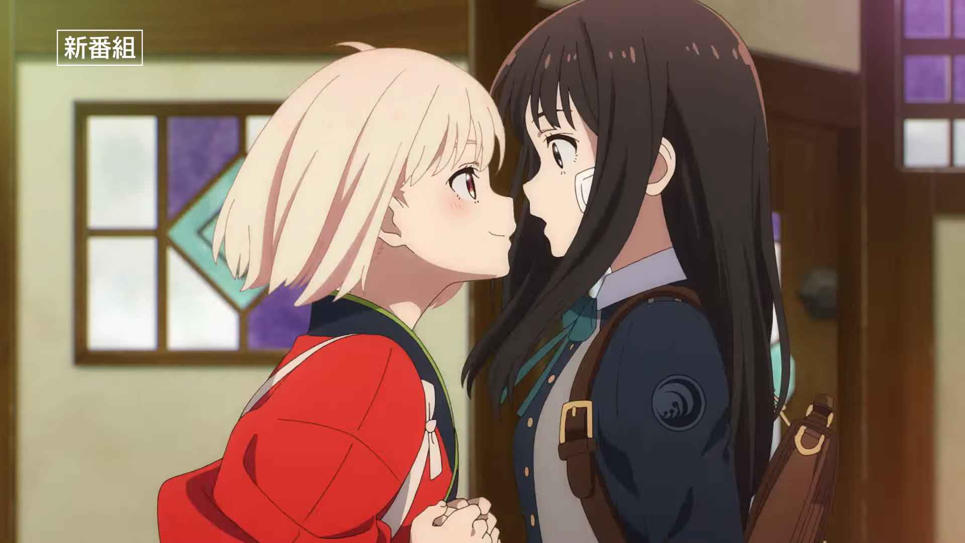
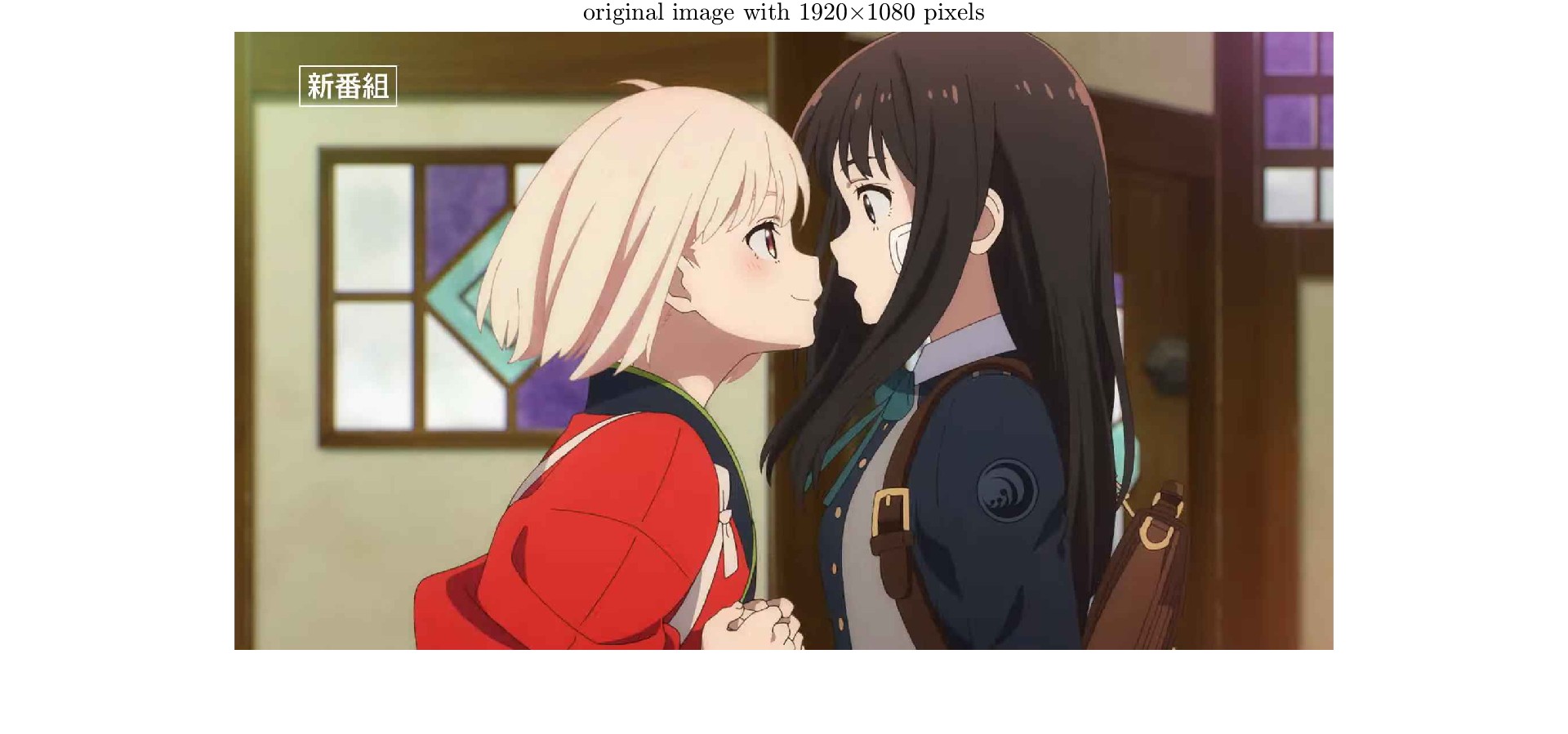
給定輸入圖片`lycoris_recoil.jpg`。<br>
```matlab
clc, clear, close all
%% read file and change data type
filename = 'lycoris_recoil.jpg';
imfinfo(filename) % image information
rare_data = imread(filename); % data type : uint8
cal_data = double(rare_data); % data type : double
size_A = size(cal_data); % size of A
imshow(cal_data/255); % imshow(RGB) with RGB in [0,1]
title(['original image with ',num2str(size_A(2)),'$\times$',num2str(size_A(1)),' pixels'],'interpreter','latex','FontSize',15);
axis equal; % maintain aspect ratio of x,y
axis off; % turn off axis
```
<br>
首先讀取圖檔,並用指令`imfinfo()`查看圖檔資訊為$1920 \times 1080$像素,位元深度(bit depth)為24位元,色型為true color,代表有3條通道(channel)分別為紅、綠、藍,每一條通道的位元深度為8位元。而圖片預設儲存的資料型態為無號(unsigned) 8位元整數(`uint8`),在計算機運算時,將其轉換為雙精度浮點數運算(`double`)。由於指令`imshow`要顯示true color影像,若是資料型態是浮點數則數值限制在$[0,1]$,因此除上$255$,將$[0, 255]$映射至$[0,1]$。
```matlab
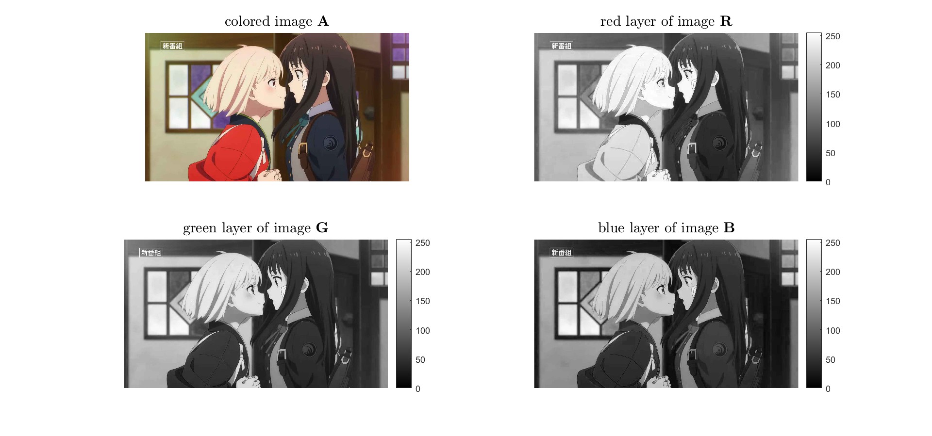
%% decompose coloered images into RGB layers
cal_data_1 = cal_data(:,:,1);
cal_data_2 = cal_data(:,:,2);
cal_data_3 = cal_data(:,:,3);
subplot(2,2,1);
imshow(cal_data/255);
title('colored image $\mathbf{A}$','interpreter','latex','FontSize',15);
subplot(2,2,2);
imshow(cal_data_1,[0,255]);
title('red layer of image $\mathbf{R}$','interpreter','latex','FontSize',15);
colorbar
subplot(2,2,3);
imshow(cal_data_2,[0,255]);
title('green layer of image $\mathbf{G}$','interpreter','latex','FontSize',15);
colorbar
subplot(2,2,4);
imshow(cal_data_3,[0,255]);
title('blue layer of image $\mathbf{B}$','interpreter','latex','FontSize',15);
colorbar
```
<br>
將true color影像的R、G、B通道分解,也就是把3維矩陣降至3個2維矩陣
$$
\mathbf{A} \in \mathbb{R}^{1080 \times 1920 \times 3} \to \mathbf{R}, \mathbf{G}, \mathbf{B} \in \mathbb{R}^{1080 \times 1920}
$$
需要注意灰階影像顯示時,預設數值範圍是$[0,1]$,因此在指令`imshow`後面要給與要對應灰階的範圍更改為$[0,255]$。
```matlab
%% singular value decomposition
[U1,S1,V1] = svd(cal_data_1);
[U2,S2,V2] = svd(cal_data_2);
[U3,S3,V3] = svd(cal_data_3);
```
分別對矩陣$\mathbf{R, G, B}$做SVD分解為$\mathbf{U}\mathbf{\Sigma} \mathbf{V}^T$的形式。
```matlab
%% plot of sigular value
sigular_value_number = min(size(S1));
x_axis = 1:sigular_value_number;
sigular_value_1 = zeros(1, length(x_axis));
sigular_value_2 = zeros(1, length(x_axis));
sigular_value_3 = zeros(1, length(x_axis));
for i = 1:sigular_value_number % take diagonal entries
sigular_value_1(1,i) = S1(i,i);
sigular_value_2(1,i) = S2(i,i);
sigular_value_3(1,i) = S3(i,i);
end
subplot(3,1,1);
semilogy(x_axis, sigular_value_1, 'LineWidth',2);
title(['sigualr value $\sigma_i$ of $\mathbf{R}$ for i = 1, 2, ...', num2str(sigular_value_number)],'interpreter','latex','FontSize',15);
xlabel('i-axis','FontSize',10);
ylabel('sigualr value \sigma_i','FontSize',10);
grid on
subplot(3,1,2);
semilogy(x_axis, sigular_value_2, 'LineWidth',2);
title(['sigualr value $\sigma_i$ of $\mathbf{G}$ for i = 1, 2, ...', num2str(sigular_value_number)],'interpreter','latex','FontSize',15);
xlabel('i-axis','FontSize',10);
ylabel('sigualr value \sigma_i','FontSize',10);
grid on
subplot(3,1,3);
semilogy(x_axis, sigular_value_3, 'LineWidth',2);
title(['sigualr value $\sigma_i$ of $\mathbf{B}$ for i = 1, 2, ...', num2str(sigular_value_number)],'interpreter','latex','FontSize',15);
xlabel('i-axis','FontSize',10);
ylabel('sigualr value \sigma_i','FontSize',10);
grid on
```
$$
\mathbf{\Sigma} = \begin{bmatrix}
\sigma_1 & \cdots & \mathbf{0} & \mathbf{0} & \cdots & \mathbf{0}\\
\vdots & \ddots & \vdots & \vdots & \ddots & \vdots\\
\mathbf{0} & \cdots & \sigma_{ 1080} & \mathbf{0} & \cdots & \mathbf{0}\\
\end{bmatrix}_{ 1080 \times 1920}, \text{ where } \sigma_1 \geq \sigma_2 \geq \cdots \geq \sigma_{1080} \geq 0
$$
矩陣$\mathbf{R, G, B}$的奇異值$\sigma_i$數值對index $i$作圖,可以發現以此張圖來說,R、G、B圖層的奇異值$\sigma_i$分布類似;需要注意$\sigma_i$數值是對數$\log$作圖,因此奇異值大小變化量劇烈,代表取足夠前$k$項的SVD的外積展開式,就幾乎可以涵蓋整張圖的所有資訊
$$
\mathbf{A} = \underbrace{\sigma_1 \mathbf{u}_1 \mathbf{v}_1^T + \sigma_2 \mathbf{u}_2 \mathbf{v}_2^T + \ldots + \sigma_k \mathbf{u}_k \mathbf{v}_k^T}_{\text{encode almost image message}} + \ldots + \sigma_{1080}\mathbf{u}_{1080}\mathbf{v}_{1080}^T, k <1080
$$
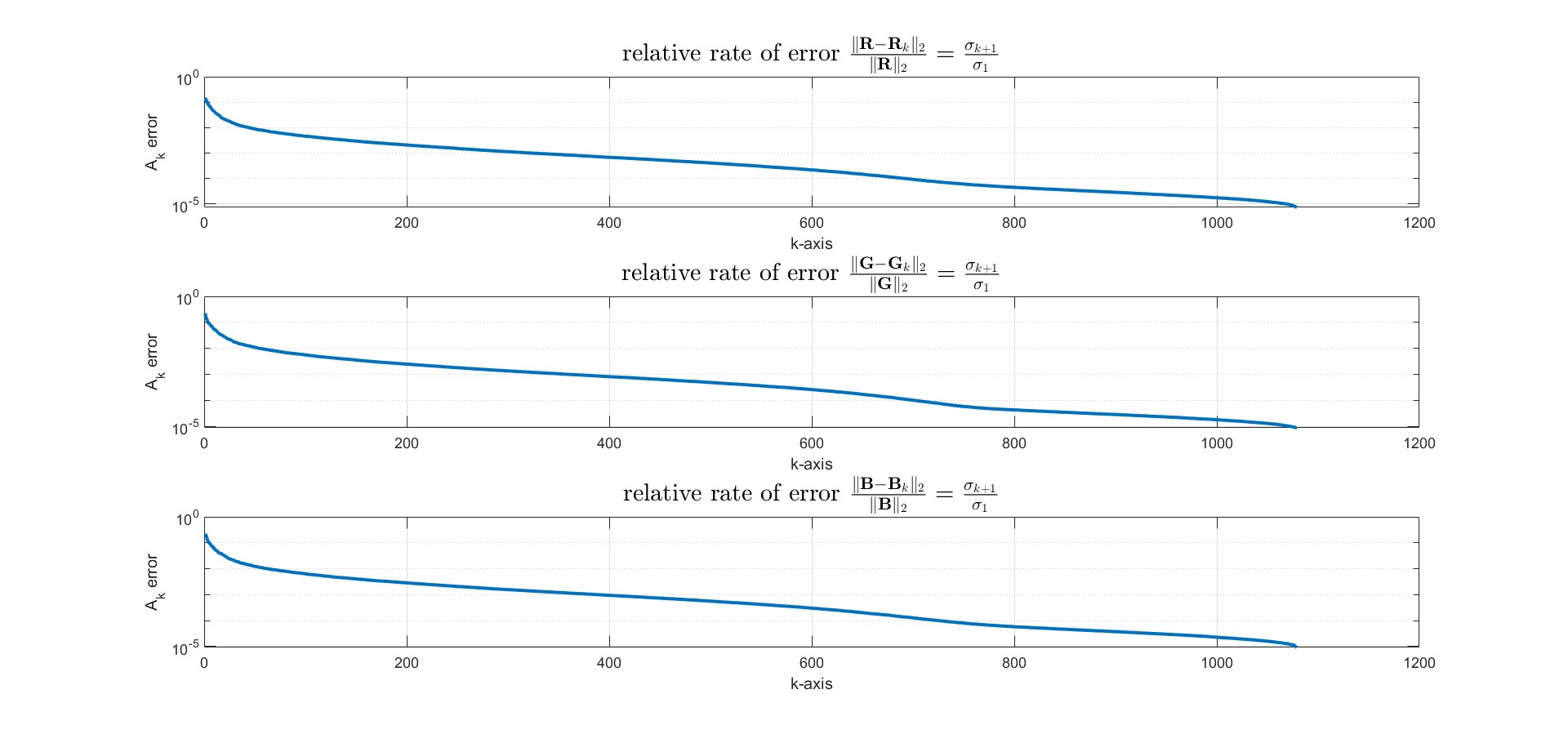
```matlab
%% minimal relative rate of error
subplot(3,1,1);
error_1 = sigular_value_1(2:end) / S1(1,1);
semilogy(x_axis(1:end-1), error_1, 'LineWidth',2);
title('relative rate of error $\frac{\| \mathbf{R} - \mathbf{R}_k \|_2}{\| \mathbf{R} \|_2} = \frac{\sigma_{k + 1}}{\sigma_1}$','interpreter','latex','FontSize',15);
xlabel('k-axis','FontSize',10);
ylabel('A_k error','FontSize',10);
grid on
subplot(3,1,2);
error_2 = sigular_value_2(2:end) / S2(1,1);
semilogy(x_axis(1:end-1), error_2, 'LineWidth',2);
title('relative rate of error $\frac{\| \mathbf{G} - \mathbf{G}_k \|_2}{\| \mathbf{G} \|_2} = \frac{\sigma_{k + 1}}{\sigma_1}$','interpreter','latex','FontSize',15);
xlabel('k-axis','FontSize',10);
ylabel('A_k error','FontSize',10);
grid on
subplot(3,1,3);
error_3 = sigular_value_3(2:end) / S3(1,1);
semilogy(x_axis(1:end-1), error_3, 'LineWidth',2);
title('relative rate of error $\frac{\| \mathbf{B} - \mathbf{B}_k \|_2}{\| \mathbf{B} \|_2} = \frac{\sigma_{k + 1}}{\sigma_1}$','interpreter','latex','FontSize',15);
xlabel('k-axis','FontSize',10);
ylabel('A_k error','FontSize',10);
grid on
```
<br>
至於這個$k$項要取多少?根據前面[數學理論](#數學理論)中矩陣之間的"距離"這個概念,在此使用norm的其中一種定義 - 2-norm來求得相對誤差值。
```matlab
%% compressed with factor of k
k = 30; % reduced to number of singlular values
S_re_1 = zeros(size_A(1),size_A(2));
S_re_2 = zeros(size_A(1),size_A(2));
S_re_3 = zeros(size_A(1),size_A(2));
for ir = 1:k
S_re_1(ir,ir) = S1(ir,ir); % compress red layer of image
S_re_2(ir,ir) = S2(ir,ir); % compress green layer of image
S_re_3(ir,ir) = S3(ir,ir); % compress blue layer of image
end
A_re_1 = U1*S_re_1*V1';
A_re_2 = U2*S_re_2*V2';
A_re_3 = U3*S_re_3*V3';
```
我選擇把R、G、B的相對誤差都限制在$2\%$以內,因此選擇$k = 31$,此時R、G、B誤差為
$$
\begin{align*}
\text{relative rate error of red layer} &= \frac{\| \mathbf{R} - \mathbf{R}_k \|_2}{\| \mathbf{R} \|_2} \approx 0.0138466 < 2\%\\
\text{relative rate error of green layer} &= \frac{\| \mathbf{G} - \mathbf{G}_k \|_2}{\| \mathbf{G} \|_2} \approx 0.0173546 < 2\%\\
\text{relative rate error of blue layer} &= \frac{\| \mathbf{B} - \mathbf{B}_k \|_2}{\| \mathbf{B} \|_2} \approx 0.0192512 < 2\%
\end{align*}
$$
```matlab
%% combine RGB layers into colored images
figure;
A_re = uint8(zeros(size_A(1), size_A(2), size_A(3)));
A_re(:,:,1) = uint8(A_re_1);
A_re(:,:,2) = uint8(A_re_2);
A_re(:,:,3) = uint8(A_re_3);
imshow(A_re);
title('compressed colored image $\mathbf{R}_k, \mathbf{G}_k,\mathbf{B}_k \to \mathbf{A}_k$ with low rank approximation','interpreter','latex','FontSize',15);
axis equal;
axis off;
```
<br>
最後合併壓縮後的$\mathbf{R, G, B}$矩陣回原來的影像。可以發現原本原本$\mathrm{rank}(\mathbf{A}) = 1080$的矩陣,現在只需要取$k = 31$,使矩陣秩數只要$\mathrm{rank}(\mathbf{A}_k) = 31$,就可以看出原本影像大部分的特徵。
```matlab
%% each RGB layers after low rank approximation
subplot(2,2,1);
imshow(A_re);
title('colored image $\mathbf{A}_k$','interpreter','latex','FontSize',15);
subplot(2,2,2);
imshow(uint8(A_re_1));
colorbar
title('red layer of image $\mathbf{R}_k$','interpreter','latex','FontSize',15);
subplot(2,2,3);
imshow(uint8(A_re_2));
colorbar
title('green layer of image $\mathbf{G}_k$','interpreter','latex','FontSize',15);
subplot(2,2,4);
imshow(uint8(A_re_3));
colorbar
title('blue layer of image $\mathbf{B}_k$','interpreter','latex','FontSize',15);
```
<br>
把R、G、B壓縮影像印出來,看個別R、G、B圖層壓縮的效果。
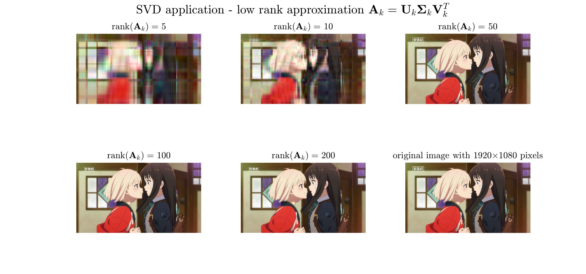
```matlab
%% comparison of different rank k
sgtitle('SVD application - low rank approximation $\mathbf{A}_k = \mathbf{U}_k\mathbf{\Sigma}_k\mathbf{V}_k^T$','interpreter','latex','FontSize',20);
k = [5,10,50,100, 200]; % number of singlular values
for i = 1:length(k)
S_re_1 = zeros(size_A(1),size_A(2));
S_re_2 = zeros(size_A(1),size_A(2));
S_re_3 = zeros(size_A(1),size_A(2));
for ir = 1:k(i)
S_re_1(ir,ir) = S1(ir,ir); % compress red layer of image
S_re_2(ir,ir) = S2(ir,ir); % compress green layer of image
S_re_3(ir,ir) = S3(ir,ir); % compress blue layer of image
end
A_re_1 = U1*S_re_1*V1';
A_re_2 = U2*S_re_2*V2';
A_re_3 = U3*S_re_3*V3';
A_re = uint8(zeros(size_A(1), size_A(2), size_A(3)));
A_re(:,:,1) = uint8(A_re_1);
A_re(:,:,2) = uint8(A_re_2);
A_re(:,:,3) = uint8(A_re_3);
subplot(2,3,i);
imshow(A_re);
title(['$\mathrm{rank}(\mathbf{A}_k) =$ ',num2str(k(i))],'interpreter','latex','FontSize',15);
end
subplot(2,3,6);
imshow(cal_data/255);
title(['original image with ',num2str(size_A(2)),'$\times$',num2str(size_A(1)),' pixels'],'interpreter','latex','FontSize',15);
```
<br>
最後寫一個`for loop`,觀察取不同$k$,也就是不同的秩數下所得到的效果,可以發現在$\mathrm{rank}(\mathbf{A}) = 100$,以目前這種顯示比例,跟原圖比較幾乎看不出有什麼區別,幾乎能保留影像大部分的特徵,而使用秩數較低的矩陣同時又能減少大量資料儲存,這就是low rank approximation在影像壓縮的應用與意義。