--- # System prepended metadata title: 【R 語言與統計資料分析】Ch5：R 繪圖與 ggplot2、plotly 實戰 tags: [R 語言與統計資料分析] --- --- title: 【R 語言與統計資料分析】Ch5：R 繪圖與 ggplot2、plotly 實戰 image: https://ppt.cc/fnT4xx@.png --- # 【R 語言與統計資料分析】Ch5：R 繪圖與 ggplot2、plotly 實戰 # 5.1 什麼是圖表? **圖表** (Charts/Graphs) 是透過視覺化手段來呈現數據、統計數字或複雜概念的工具，旨在**簡化資訊**並**凸顯資料間的結構、趨勢與差異**。 ## 5.1.1 數據圖表 **數據圖表** (Chart) 為帶有量化數據的圖形或圖案，即具圖像化的資料表，用以使讀者方便理解大量數據，以及數據之間的關係。如：圓餅圖、長條圖、直方圖、折線圖等各式統計圖表。

圓餅圖就是一種數據圖表

## 5.1.2 資訊圖表 **資訊圖表** (Infographics) 其英文顧名思義為「資訊」 (information) 以及「圖表」(graphic) 所結合而成的複合單字，指資料、資訊或知識的視覺化表現形式。目的為清楚準確的解釋或表達甚為複雜且大量的資訊，被廣泛應用在各式各樣的文件檔案上。

由中央氣象署發布的資訊圖表

## 5.1.3 圖表的 TOP 原則 #### Target（對象）：圖表是給誰看的？我們必須優先確認受眾是誰，再進一步決定圖表的呈現的深度與複雜度。在設計時，或許可以透過顏色、標記或直接在標題寫出結論，引導受眾在最短時間內抓到重點。 #### Object（目的）：希望傳達出什麼訊息或達成什麼目的？釐清目的能決定圖表的類型選擇與敘事方式，比如針對不同的資料型態，使用對應的圖表進行敘事；對主管報告，優先提供決策所需的資訊等等。 #### Place（場合）：圖表用什麼形式展現？圖表呈現的場合是相當重要的，會直接影響圖表的「視覺設計細節」，如: 放在正式文件、內部會議簡報、社群媒體文案，還是 E-mail 附件等等。若是現場簡報，圖表應簡潔並由講者輔助；若是電子文件，圖表必須具備自我解釋能力（Self-explanatory）。 # 5.2 在 R 中用 `Base` 繪製圖表 ## 5.2.1 用 `par()` 開始處理畫布 #### 用 `mar` 控制邊界

mar = c(下, 左, 上, 右)

```r # mar = c(下, 左, 上, 右) # 邊界超小，圖片超大 par(mar = c(1,1,1,1) ) boxplot(iris$Sepal.Width ~ iris$Species, ylab = "Sepal width (cm)", main = "Anderson's Iris Data") # 邊界超大，圖片超小 par(mar = c(15,15,15,15) ) boxplot(iris$Sepal.Width ~ iris$Species, ylab = "Sepal width (cm)", main = "Anderson's Iris Data") ``` #### 用 `mfcol` 與 `mfrow` 來合併繪圖在進行圖片繪製時，常常會需要將多張圖片放置在一起排版，此事就可以使用 `mfcol` 與 `mfrow` 來進行版面的規劃。`mfcol` 為依照「**直行**」的方向進行排列，而 `mfrow` 為依照「**橫列**」的方向進行排列。 ```r # mfcol 的範例 par(mfcol = c(3,2)) #指形成一個 3x2 的繪圖矩陣 boxplot(iris$Sepal.Width ~ iris$Species, main = "Plot A") boxplot(iris$Sepal.Width ~ iris$Species, main = "Plot B") boxplot(iris$Sepal.Width ~ iris$Species, main = "Plot C") boxplot(iris$Sepal.Width ~ iris$Species, main = "Plot D") boxplot(iris$Sepal.Width ~ iris$Species, main = "Plot E") boxplot(iris$Sepal.Width ~ iris$Species, main = "Plot F") ``` ![image](https://hackmd.io/_uploads/B1NhyV4FWl.png =70%x) ```r # mfrow 的範例 par(mfrow = c(3,2)) #指形成一個 3x2 的繪圖矩陣 boxplot(iris$Sepal.Width ~ iris$Species, main = "Plot A") boxplot(iris$Sepal.Width ~ iris$Species, main = "Plot B") boxplot(iris$Sepal.Width ~ iris$Species, main = "Plot C") boxplot(iris$Sepal.Width ~ iris$Species, main = "Plot D") boxplot(iris$Sepal.Width ~ iris$Species, main = "Plot E") boxplot(iris$Sepal.Width ~ iris$Species, main = "Plot F") ``` ![image](https://hackmd.io/_uploads/B100JVEYWe.png =70%x) 在執行 `par(mfcol = c(3,2))` 或 `par(mfrow = c(3,2))` 後，畫圖的布局就已被更改，下次若要繪圖，一樣會從繪圖區的左上角依序繪製。若要恢復成單一圖表狀態，可使用 `par(mfcol = c(1,1))` 更改布局或是使用 `dev.off()` 來恢復成預設狀態。 #### 用 `layout` 做不對稱排版除了對稱的排版之外，我們也會使用不對稱的排版。舉例來說，我們可能會想要凸顯某一張圖作為重點，而其他圖片作為此議題的補充，此時就會想把重點圖片作放大，其餘部分就可以做為陪襯。關於 `layout()` 函數的應用，與矩陣呈現的形式息息相關，我們直接以實際案例作介紹: ``` matrix(c(1,1,2,3),2,2) #先看矩陣長什麼樣子 layout(matrix(c(1,1,2,3),2,2)) boxplot(iris$Sepal.Width ~ iris$Species, main = "Plot A") boxplot(iris$Sepal.Width ~ iris$Species, main = "Plot B") boxplot(iris$Sepal.Width ~ iris$Species, main = "Plot C") ```

用 layout() 做不對稱排版

## 5.2.3 圖形基本設定在 `par()` 中，我們也可以控制畫圖的細節部分，如線條樣式、顏色等等，此外也可以在如 `plot()` 等繪圖函數中進行設定。 - `lwd`：線條粗度 - `type`：點與點間連線樣式 - `lty`：線條樣式 - `cex`：字體大小 - `pch`：點的樣式 - `font`：控制粗體斜體 - `col`：顏色控制，

R 繪圖設定代碼

在色彩方面，可以使用不同的代碼，在 R 中都可以去解讀: - 文字名稱：如 "red"、"skyblue"、"gold"。R 內建超過 600 種顏色名稱（可用 `colors()` 查看）。 - 十六進位碼：如 "#FF5733"，適合與網頁設計或品牌色對接。 - 數字代號：1=黑, 2=紅, 3=綠, 4=藍 ...。 ```r # 產生測試數據 x <- 1:10 y <- x^2 # 繪圖 plot(x, y, main = "Analysis", # main xlab = "(sec)", # xlab ylab = "(Value)", # ylab col = "darkorange", # col pch = 21, # pch (使用帶邊框的圓) bg = "yellow", # 配合 pch=21 的填充色 cex = 2, # cex (放大點的大小) type = "b", # 同時畫點和線 (both) lty = 2, # lty (使用虛線) lwd = 2) # 加粗線條 ```

## 5.2.3 基本繪圖補充在 [Ch2](https://hackmd.io/@wwwh0225/H1ImLs9rZg#24-%E6%95%B8%E6%93%9A%E6%B4%9E%E5%AF%9F%EF%BC%9A%E6%95%98%E8%BF%B0%E7%B5%B1%E8%A8%88%E8%88%87%E7%B9%AA%E5%9C%96%E6%87%89%E7%94%A8) 中，我們已有稍微提到繪圖相關的程式碼，我們在此做一些小補充。當我們畫好一張圖後，若要進行修改，在 R 中是比較困難的。在 R 中的繪圖是類似「疊圖」的方式進行繪製，因此若一步做錯，整張圖就需要重新再繪製一次。讓我們以與前面章節同樣的一張圖做延伸:

- 加上「**點**」：`points(x,y)` ```r points(6,60,pch = 11) ``` - 加上「**線段**」：`lines(x,y)` ```r #畫上兩點 x1 <- c(2,4) y1 <- c(80,80) points(x1,y1 ,pch = 15) #連起來 lines(x1,y1) ``` - 加上「**文字**」：`text(x,y,labels)` ```r text(8,20,"GOOD") #在 (8,20) 寫字 ``` - 加上「**直線**」：`abline(a,b)` 為 $y=a+bx$ 的直線 ```r #加上 45度直線 abline(1,1) #加上水平線 abline(h = 50) #加上垂直線 abline(v = 5) ```

## 5.2.4 中文字體處理在進行 R 語言中的繪圖時，中文字體有時會出現顯示異常的情形，我們以下列程式碼為例: ```r curve(dnorm(x, mean = 0, sd = 1), from = -3, to = 3, col = "blue", # 線條顏色 lwd = 2, # 線條寬度 main = "標準常態分佈 N(0,1) pdf", xlab = "z 分數", ylab = "機率密度") ```

有時候中文字體會顯示不出來

這時，我們必須強制指定一個中文字體 (`family`)，讓 R 語言可以正確地進行渲染編碼。 ```r # 以 Mac 電腦為例 curve(dnorm(x, mean = 0, sd = 1), from = -3, to = 3, col = "blue", # 線條顏色 lwd = 2, # 線條寬度 main = "標準常態分佈 N(0,1) pdf", xlab = "z 分數", ylab = "機率密度", family = "STKaiti") # 此處填寫字體名稱 ```

指定中文字體後就可以正確顯示

找尋字體名稱的方法，可以參考[此網址](https://r-lover.com/tutorial/visualization/chinese-in-ggplot2/#%E5%9C%A8Windows%E7%B3%BB%E7%B5%B1%E4%B8%AD%E5%91%88%E7%8F%BE%E4%B8%AD%E6%96%87%E5%AD%97%E9%AB%94)。 # 5.3 用 `ggplot2` 套件進行繪圖 `ggplot2` 是由 Hadley Wickham 開發，基於 Leland Wilkinson 的「圖形語法」(Grammar of Graphics) 理論，而它的核心思想是：任何圖表都可以拆解成相同的基本組件。

ggplot2 的圖層概念

繪製一張 ggplot2 圖表就像疊加投影片的圖層，基本概念如下: $$\text{ggplot}(\text{data}) + \text{aes}(\text{mappings}) + \text{geom_xxx}()$$ 若要使用 `ggplot2` 套件，需要在 R 中先下載此套件: ```r # 下載套件 install.packages("ggplot2") ``` ```r # 呼叫套件 library(ggplot2) ``` 在 `ggplot2` 中，許多的設定都已被模組化寫好，讓我們以實際案例來介紹 `ggplot2` 的強大之處。 ## 5.3.1 直方圖我們使用 `geom_histogram` 來繪製直方圖。我們在此使用美國高中生的身高資料，請先載入套件後，使用 `heights` 資料集。由於 `heights` 資料集內的身高為英吋單位，我們在此先轉換為公分單位。 ``` library(dslabs) #載入套件中的資料集 # 如果沒有此套件，請執行 install.packages("dslabs") # 觀看查詢前 6 筆資料 heights$height_cm <- heights$height * 2.54 #英吋換成公分 head(heights) ```

身高資料 (cm)

接著，我們將男生與女生的身高分佈統一畫在同一張圖內。這跟先前所使用的 `par()` 設定不同，`par()` 的並圖是分別畫完一張圖後放入設定好的空間；而 `ggplot2` 是在內部會依據類別的數量自動規劃圖形的合併與呈現規劃。此處的 `facet_wrap` 與 `fill = sex` 就是扮演這個角色。由於中文字型需要被另外設定，我們需要在 `theme` 中加入指定字體的程式碼，如：`element_text(family = "PingFang TC")`，各台電腦所要對應的字體就如同前述，大家可以測試看看。 ```r ggplot(heights, aes(x = height_cm, fill = sex)) + geom_histogram(binwidth = 5, color = "black", alpha = 0.7) + # 設定 binwidth 和透明度 facet_wrap(~ sex, scales = "free_y") + # 依據 sex 拆圖，scales="free_y" 讓y軸範圍各自調整 labs( title = "男生與女生身高分佈直方圖", subtitle = "分別顯示", x = "身高 (cm)", y = "人數 (Count)", fill = "性別" ) + theme_minimal() + scale_fill_manual(values = c("Female" = "salmon", "Male" = "skyblue")) + # 手動設定顏色 theme(text = element_text(family = "PingFang TC")) # 設定文字字體 ```

依照性別繪製直方圖

## 5.3.2 長條圖在 `ggplot2`，我們使用 `geom_bar` 來繪製長條圖，以下使用 `mpg` 資料集，裡面搜集了許多關於不同品牌汽車油耗的資料。 ```r # 觀察前 6 筆資料 head(mpg) ``` 依照汽車品牌繪製長條圖，由於某些品牌名稱較長，我們設定品牌名稱會旋轉 45 度後呈現： ```r # 長條圖 ggplot(mpg, aes(x = manufacturer)) + geom_bar(fill = "steelblue") + theme_minimal() + labs(title = "各品牌汽車數量長條圖", x = "品牌", y = "數量") + theme(axis.text.x = element_text(angle = 45, hjust = 1), text = element_text(family = "PingFang TC")) # 設定文字字體 ```

汽車品牌長條圖

若我們想要依照不同車型上色，一樣是在 `aes()` 中加入 `fill = class`。 ```r # 以車型分類 ggplot(mpg, aes(x = manufacturer, fill = class)) + geom_bar() + scale_fill_brewer(palette = "Set3")+ # 顏色調色盤 theme_minimal() + labs(title = "各品牌之車型組成長條圖", x = "品牌", y = "數量", fill = "車型類別") + theme(axis.text.x = element_text(angle = 45, hjust = 1), text = element_text(family = "PingFang TC")) # 設定文字字體 ```

汽車品牌長條圖 - 以類別分組

## 5.3.3 散佈圖在 ggplot 繪製散佈圖也是十分簡單，只要將 x 軸與 y 軸對應的座標點匯入即可： ``` # 散佈圖 ggplot(iris, aes(x = Sepal.Length, y = Sepal.Width, color = Species)) + geom_point(size = 3) + # 設定點的大小 theme_minimal() + # 使用簡潔主題 labs(title = "Iris 鳶尾花花萼長寬散佈圖", x = "花萼長度 (Sepal Length)", y = "花萼寬度 (Sepal Width)") + theme(text = element_text(family = "PingFang TC")) # 設定文字字體 ```

鳶尾花散佈圖

如果我們想要把「圖例」移到下方怎麼辦呢? 善用 ChatGPT、Gemini 等工具!!! ```r # AI 修訂 ggplot(iris, aes(x = Sepal.Length, y = Sepal.Width, color = Species)) + geom_point(size = 3) + # 設定點的大小 theme_minimal() + # 使用簡潔主題 labs(title = "Iris 鳶尾花花萼長寬散佈圖", x = "花萼長度 (Sepal Length)", y = "花萼寬度 (Sepal Width)") + theme(legend.position = "bottom") #圖例放在最下面 ```

鳶尾花散佈圖

此外，`ggplot2` 也可以很簡單地插入變數間的迴歸線，用以表示資料之間的關聯趨勢。 ```r # 加入預測線 ggplot(iris, aes(x = Sepal.Length, y = Sepal.Width, color = Species)) + geom_point(size = 3) + # 設定點的大小 theme_minimal() + # 使用簡潔主題 labs(title = "Iris 鳶尾花花萼長寬散佈圖", x = "花萼長度 (Sepal Length)", y = "花萼寬度 (Sepal Width)") + theme(text = element_text(family = "PingFang TC"))+ # 設定文字字體 geom_smooth(method = "lm", color = "black") # 畫出一條整體的黑色預測線 ```

鳶尾花散佈圖與迴歸直線

先前，我們曾介紹 `pair()` 函數，用來直接繪製所有資料兩兩間的關係，在 `ggplot2` 的世界裡，我們可以套用 `GGally` 套件，可以給予我們更豐富的分析視角。 `GGally` 除了提供散佈圖之外，還會回報變數間的相關係數、核密度估計 (kernel density estimation, KDE) 以及長條圖及盒狀圖等圖形。 ```r # 安裝並載入套件 install.packages("GGally") ``` ```r library(GGally) # 記得執行 library(ggplot2) # 記得執行 ggpairs(iris, aes(color = Species, alpha = 0.5), title = "GGally 矩陣圖：包含相關係數與分佈") + theme_bw() + theme(text = element_text(family = "PingFang TC")) # 設定文字字體 ``` ![image](https://hackmd.io/_uploads/rJBUCmEFZe.png) ## 5.3.4 熱力圖熱力圖 (Heatmap) 是一種用顏色表示數值大小的二維圖表，適合用在矩陣型資料 (如：時間 × 地點 → 銷售額)、數值變數之間的相關係數等情境。我們以 `mtcars` 資料集為例，顯示 32 款不同汽車的性能數據: ```r # 先閱讀資料 head(mtcars) ``` 我們希望觀察資料間相關係數的強弱關係，透過熱力圖將相關係數矩陣視覺化: ```r library(ggplot2) library(reshape2) # 若無此套件，請記得下載install.packages("reshape2") # 取數值欄位 num_mtcars <- Filter(is.numeric, mtcars) # 計算相關係數 cor_mat <- cor(num_mtcars) # 用 melt 轉長表 long_df <- melt(cor_mat) print(head(long_df)) # 畫 heatmap ggplot(long_df, aes(x = Var1, y = Var2, fill = value)) + geom_tile() + scale_fill_gradient2(low="blue", mid="white", high="red", limits=c(-1,1)) + labs(title="mtcars Correlation Heatmap", fill="Correlation") + theme_minimal() ```

相關係數熱力圖

## 5.3.4 折線圖折線圖是分析時間資料常會用到的圖形，我們以航空業資料 `AirPassengers` 來做介紹，我們先將其轉為 `dataframe` 格式後再行繪圖。 ```r df_air <- data.frame( Year = as.numeric(floor(time(AirPassengers))), Month = as.numeric(cycle(AirPassengers)), Passengers = as.numeric(AirPassengers) ) # 將月份數字轉為英文縮寫 (如 1 轉為 Jan) df_air$Month_Name <- factor(month.abb[df_air$Month], levels = month.abb) head(df_air) ```

依照年份、月份分類的航空業旅客資料

接下來，讓我們依照年分畫出對應的折線圖: ```r # 折線圖 ggplot(df_air, aes(x = Month_Name, y = Passengers, group = Year, color = factor(Year))) + geom_line(size = 1) + # 畫出折線 geom_point(size = 1.5) + # 加入數據點，方便觀察每個月的數值 scale_color_viridis_d() + # 使用 viridis 調色盤，顏色過渡較自然且專業 theme_minimal() + # 使用簡潔主題 labs( title = "AirPassengers 每月乘客數年度變化圖", subtitle = "觀察各月份在不同年份的增長趨勢", x = "月份", y = "乘客數", color = "年份" # 圖例名稱 ) + theme( legend.position = "right", # 圖例放在右側 plot.title = element_text(face = "bold", size = 14), text = element_text(family = "PingFang TC") ) ```

依照年份、月份分類的航空業旅客數折線圖

## 5.3.5 標題位置調整從我們畫的這幾張圖中，可以看到 `ggplot2` 對於圖表標題的預設是於左上方開始進行呈現。但我們常常會希望進行標題置中，那此時就需要於 `theme()` 中設定 `plot.title = element_text(hjust = 0.5)`，`hjust = 0.5` 是置中的意思，預設的位置是在 0。 ```r # 散佈圖 ggplot(iris, aes(x = Sepal.Length, y = Sepal.Width, color = Species)) + geom_point(size = 3) + # 設定點的大小 theme_minimal() + # 使用簡潔主題 labs(title = "Iris 鳶尾花花萼長寬散佈圖", x = "花萼長度 (Sepal Length)", y = "花萼寬度 (Sepal Width)") + theme(text = element_text(family = "PingFang TC"), # 設定文字字體 plot.title = element_text(hjust = 0.5)) # 置中標題 ```

標題置中的鳶尾花散佈圖

# 5.4 `plotly` 套件應用 `plotly` 是一個基於 JavaScript (plotly.js) 的繪圖庫，就像是一個儀表板一樣，我們可以透過滑鼠與資料進行互動，或是對圖表進行縮放等直觀性操作。 ```r # 下載套件 install.packages("plotly") ``` ## 5.4.1 `plotly` 內建寫法我們可以透過 `plot_ly()` 函數去進行圖表的繪製，但這又得讓我們重新學一個繪圖的語法。 ```r plot_ly(data = iris, x = ~Sepal.Length, y = ~Sepal.Width, color = ~Species, type = "scatter", mode = "markers") ``` ## 5.4.1 使用 `ggplotly` 進行轉換在 R 語言中，`plotly` 最強大的地方在於能透過 `ggplotly()` 函數與 `ggplot2` 無縫接軌。我們只需要照常繪製 `ggplot2` 圖形，再用 `ggplotly()` 包起來，靜態圖瞬間變成互動圖。

ggplotly

```r # 範例1 library(ggplot2) library(plotly) # 先畫一個標準的 ggplot p <- ggplot(iris, aes(x = Sepal.Length, y = Sepal.Width, color = Species)) + geom_point() + theme_minimal() # 轉化為互動模式 ggplotly(p) ``` ```r # 範例2 library(ggplot2) library(plotly) # 折線圖轉為 plotly lp <- ggplot(df_air, aes(x = Month_Name, y = Passengers, group = Year, color = factor(Year))) + geom_line(size = 1) + # 畫出折線 geom_point(size = 1.5) + # 加入數據點，方便觀察每個月的數值 scale_color_viridis_d() + # 使用 viridis 調色盤，顏色過渡較自然且專業 theme_minimal() + # 使用簡潔主題 labs( title = "AirPassengers 每月乘客數年度變化圖", subtitle = "觀察各月份在不同年份的增長趨勢", x = "月份", y = "乘客數", color = "年份" # 圖例名稱 ) + theme( legend.position = "right", # 圖例放在右側 plot.title = element_text(face = "bold", size = 14), text = element_text(family = "PingFang TC") ) ggplotly(lp) ``` # 5.5 盡信書，不如無書 ## 5.5.1 Y 軸的陷阱我們在進行資料時，目的就是希望能夠更直觀的去認識資料，但有時總是會有一些「**狀況**」是我們身為圖表繪製者以及讀者都要去注意的。 #### 折線圖的案例

不同 Y 軸起點對視覺造成的影響

``` # 安裝套件（如未安裝） # install.packages("patchwork") library(ggplot2) library(patchwork) #如未安裝，請執行 install.packages("patchwork") # 範例資料 df <- data.frame( year = 2015:2022, value = c(100, 102, 103, 105, 104, 106, 107, 108) ) # 圖 1：Y 軸截斷 p1 <- ggplot(df, aes(x = year, y = value)) + geom_line(linewidth = 1) + geom_point(size = 3) + scale_y_continuous(limits = c(98, 106)) + labs( title = "Y 軸截斷，成長被誇大", x = "年份", y = "數值" ) + theme_minimal() # 圖 2：完整 Y 軸 p2 <- ggplot(df, aes(x = year, y = value)) + geom_line(linewidth = 1) + geom_point(size = 3) + scale_y_continuous(limits = c(0, 110)) + labs( title = "完整期間 + Y 軸從 0 開始", x = "年份", y = "數值" ) + theme_minimal() # 使用 patchwork 並排 p1 + p2 ``` #### 長條圖的案例

不同 Y 軸起點對視覺造成的影響

```r # 載入套件 library(ggplot2) library(patchwork) # 建立資料 df <- data.frame( 城市 = c("桃園市", "新北市", "台南市", "高雄市", "台中市", "台北市"), COVID盛行率 = c(301, 300, 285, 275, 271, 223) ) # 統一顏色 bar_color <- "#2c7fb8" # 圖 1：完整 Y 軸從 0 開始 p1 <- ggplot(df, aes(x = reorder(城市, -COVID盛行率), y = COVID盛行率)) + geom_col(fill = bar_color) + geom_text(aes(label = COVID盛行率), vjust = -0.5) + scale_y_continuous(limits = c(0, 320)) + labs( title = "Y 軸從 0 開始", x = "城市", y = "盛行率 (每十萬人)" ) + theme_minimal() + theme(text = element_text(family = "PingFang TC")) # 圖 2：Y 軸從 200 開始（截斷） p2 <- ggplot(df, aes(x = reorder(城市, -COVID盛行率), y = COVID盛行率)) + geom_col(fill = bar_color) + geom_text(aes(label = COVID盛行率), vjust = -0.5) + coord_cartesian(ylim = c(200, 320)) + # ← 改這裡 labs( title = "Y 軸從 200 開始（截斷）", x = "城市", y = "盛行率 (每十萬人)" ) + theme_minimal() + theme(text = element_text(family = "PingFang TC")) # 並排 p1 + p2 ``` ## 5.5.2 不要使用雙 Y 軸在資料視覺化中，很多人會想把兩組數據放在同一張圖上，使用雙 Y 軸。然而，這種做法通常會**帶來誤導與理解成本**。以下是三個主要原因： 1. 容易製造「假相關」 2. 比例可被任意操弄 3. 增加讀者認知負擔

雙軸圖與並排的差別

資料來源：《Google必修的圖表簡報術》，商業周刊出版

# 參考資料 1. 陳旭昇(2024)，資料分析的統計學基礎:使用R語言，東華書局 2. 林建甫 Jeff Lin(2020)，[R 資料科學與統計](https://bookdown.org/jefflinmd38/r4biost) 3. Gareth James, Daniela Witten, Trevor Hastie, Robert Tibshirani. (2017). An Introduction to Statistical Learning: With Applications in R. New York: Springer. 4. 陳基國(2024). 基礎統計與R語言. 台北：五南圖書出版股份有限公司 5. 劉奕酉(2022)。[【數據思維】Chart.Guide 視覺化圖表的學習網站，告訴你如何正確的選擇與使用圖表？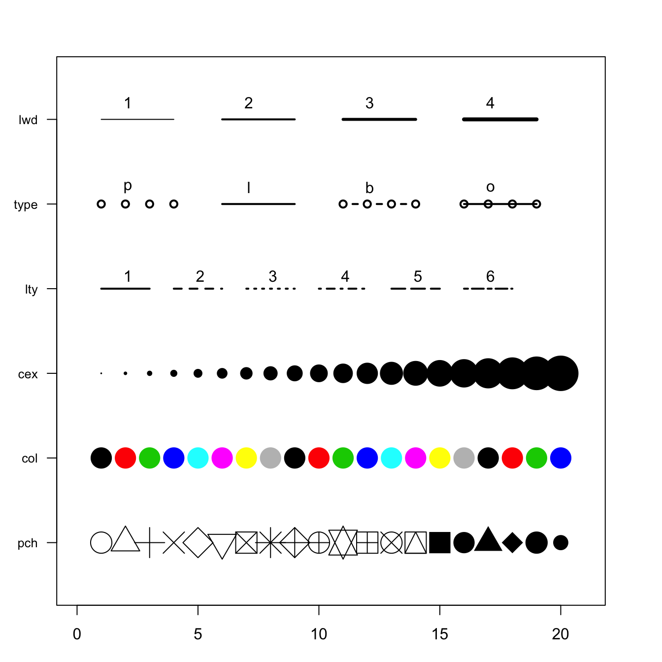](https://vocus.cc/article/61d65794fd8978000153e662) 6. Phillips(2026). [YaRrr! The Pirate’s Guide to R](https://nathanieldphillips-yarrr.share.connect.posit.cloud/)