---
# System prepended metadata
title: Ecossistema Científico
tags: [talk]
---
---
title: Ecossistema Científico
tags: talk
description: View the slide with "Slide Mode".
slideOptions:
transition: fade
theme: sky
---
## O Ecossistema Científico no Python
```python
import numpy as np
import scipy as sp
import matplotlib as mpl
```


 slides: `https://hackmd.io/@melissawm/Hyqq6d4N8`
---
### Por que estou falando disso?
slides: `https://hackmd.io/@melissawm/Hyqq6d4N8`
---
### Por que estou falando disso?
 ---
### Por que estou falando disso?
---
### Por que estou falando disso?
 ---
### Computação Científica
---
### Computação Científica
 ---
### Histórico
- BLAS (1979) - especificação de rotinas de baixo nível para operações comuns de álgebra linear
- LAPACK
- MATLAB
- Python
- Numeric/Numarray
- NumPy (2005)
---
### NumPy: a base da computação científica no Python
- objeto `ndarray` (array homogêneo n-dimensional)
- capacidade de **broadcasting**
- funções matemáticas padrão com capacidade de vetorização
- ferramentas para a integração de código C/C++ e Fortran
- álgebra linear, transformadas de Fourier, gerador de números aleatórios
---
---
### Histórico
- BLAS (1979) - especificação de rotinas de baixo nível para operações comuns de álgebra linear
- LAPACK
- MATLAB
- Python
- Numeric/Numarray
- NumPy (2005)
---
### NumPy: a base da computação científica no Python
- objeto `ndarray` (array homogêneo n-dimensional)
- capacidade de **broadcasting**
- funções matemáticas padrão com capacidade de vetorização
- ferramentas para a integração de código C/C++ e Fortran
- álgebra linear, transformadas de Fourier, gerador de números aleatórios
---
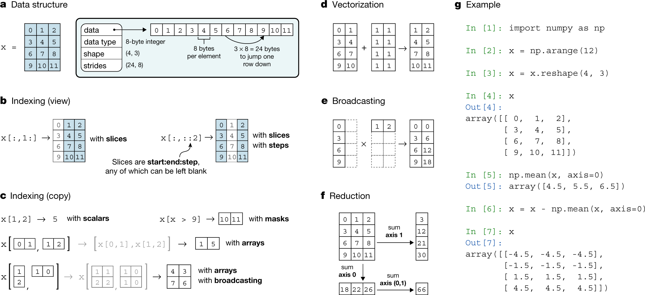
 *Fonte: Harris et al., "Array Programming with NumPy", Nature volume 585, pages 357–362 (2020)*
---
### Conceitos básicos: Vetorização
Vetorização é a capacidade de expressar operações em arrays sem especificar o que acontece com cada elemento individual (em outras palavras: sem usar loops!)
- Código vetorizado é mais conciso e legível
- O código fica (ligeiramente) mais parecido com a notação matemática
- Mais rápido (usa operações otimizadas em C/Fortran)
---
### Vetorização: Exemplo 1
```ipython
In [1]: v = [i for i in range(1000)]
In [2]: %timeit w = [i**2 for i in v]
235 µs ± 9.64 µs per loop (mean ± std. dev. of 7 runs, 1000 loops each)
In [3]: v_np = np.arange(1000)
In [4]: %timeit w_np = v_np**2
1.27 µs ± 39.6 ns per loop (mean ± std. dev. of 7 runs, 1000000 loops each)
```
---
### Como isso acontece?
As arrays do NumPy são eficientes porque
- são compatíveis com as rotinas de álgebra linear escritas em C/C++ ou Fortran
- são *views* de objetos alocados por C/C++, Fortran e Cython
- as operações vetorizadas em geral evitam copiar arrays desnecessariamente
---
*Fonte: Harris et al., "Array Programming with NumPy", Nature volume 585, pages 357–362 (2020)*
---
### Conceitos básicos: Vetorização
Vetorização é a capacidade de expressar operações em arrays sem especificar o que acontece com cada elemento individual (em outras palavras: sem usar loops!)
- Código vetorizado é mais conciso e legível
- O código fica (ligeiramente) mais parecido com a notação matemática
- Mais rápido (usa operações otimizadas em C/Fortran)
---
### Vetorização: Exemplo 1
```ipython
In [1]: v = [i for i in range(1000)]
In [2]: %timeit w = [i**2 for i in v]
235 µs ± 9.64 µs per loop (mean ± std. dev. of 7 runs, 1000 loops each)
In [3]: v_np = np.arange(1000)
In [4]: %timeit w_np = v_np**2
1.27 µs ± 39.6 ns per loop (mean ± std. dev. of 7 runs, 1000000 loops each)
```
---
### Como isso acontece?
As arrays do NumPy são eficientes porque
- são compatíveis com as rotinas de álgebra linear escritas em C/C++ ou Fortran
- são *views* de objetos alocados por C/C++, Fortran e Cython
- as operações vetorizadas em geral evitam copiar arrays desnecessariamente
---
 *Fonte: Harris et al., "Array Programming with NumPy", Nature volume 585, pages 357–362 (2020)*
---
### Vetorização: Exemplo 2
```ipython
In [1]: import numpy as np
In [2]: v = np.array([1, 2, 3, 4])
In [3]: u = np.array([2, 4, 6, 9])
In [4]: u+v
Out[4]: array([ 3, 6, 9, 13])
In [5]: np.dot(u, v)
Out[5]: 64
In [6]: u.dtype, type(u)
Out[6]: (dtype('int64'), numpy.ndarray)
```
---
### Vetorização: Exemplo 3
```ipython
In [1]: A = np.array([[1, 2, 3],
...: [4, 5, 6],
...: [7, 8, 9]])
In [2]: A.T
Out[2]:
array([[1, 4, 7],
[2, 5, 8],
[3, 6, 9]])
In [3]: A.shape, u.shape
Out[3]: ((3, 3), (4,))
In [4]: A.ndim
Out[4]: 2
In [5]: u.ndim
Out[5]: 1
```
---
### (O que são essas dimensões?)
*Fonte: Harris et al., "Array Programming with NumPy", Nature volume 585, pages 357–362 (2020)*
---
### Vetorização: Exemplo 2
```ipython
In [1]: import numpy as np
In [2]: v = np.array([1, 2, 3, 4])
In [3]: u = np.array([2, 4, 6, 9])
In [4]: u+v
Out[4]: array([ 3, 6, 9, 13])
In [5]: np.dot(u, v)
Out[5]: 64
In [6]: u.dtype, type(u)
Out[6]: (dtype('int64'), numpy.ndarray)
```
---
### Vetorização: Exemplo 3
```ipython
In [1]: A = np.array([[1, 2, 3],
...: [4, 5, 6],
...: [7, 8, 9]])
In [2]: A.T
Out[2]:
array([[1, 4, 7],
[2, 5, 8],
[3, 6, 9]])
In [3]: A.shape, u.shape
Out[3]: ((3, 3), (4,))
In [4]: A.ndim
Out[4]: 2
In [5]: u.ndim
Out[5]: 1
```
---
### (O que são essas dimensões?)
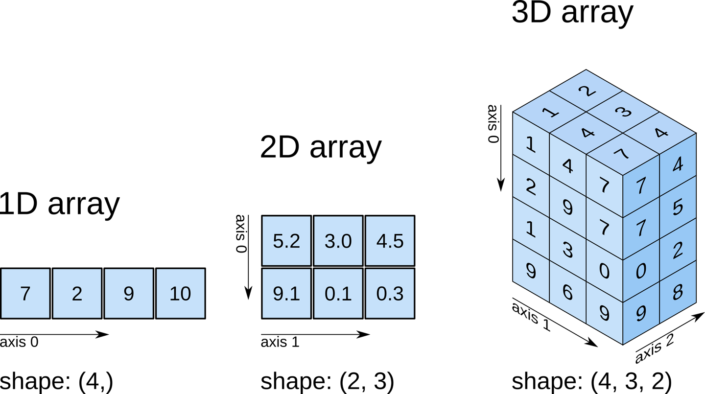 https://www.oreilly.com/library/view/elegant-scipy/9781491922927/ch01.html
---
### Vetorização: Exemplo 4
```ipython
In [6]: A[0, :]
Out[6]: array([1, 2, 3])
In [7]: A.sum()
Out[7]: 45
In [8]: A.sum(axis=0)
Out[8]: array([12, 15, 18])
In [9]: A.sum(axis=1)
Out[9]: array([ 6, 15, 24])
```
---
### Vetorização: Exemplo 5
```ipython
In [1]: x = np.arange(-np.pi, np.pi, np.pi/8)
In [2]: x
Out[2]:
array([-3.14159265, -2.74889357, -2.35619449, -1.96349541, -1.57079633,
-1.17809725, -0.78539816, -0.39269908, 0. , 0.39269908,
0.78539816, 1.17809725, 1.57079633, 1.96349541, 2.35619449,
2.74889357])
In [3]: np.sin(x)
Out[3]:
array([-1.22464680e-16, -3.82683432e-01, -7.07106781e-01, -9.23879533e-01,
-1.00000000e+00, -9.23879533e-01, -7.07106781e-01, -3.82683432e-01,
0.00000000e+00, 3.82683432e-01, 7.07106781e-01, 9.23879533e-01,
1.00000000e+00, 9.23879533e-01, 7.07106781e-01, 3.82683432e-01])
```
---
### Broadcasting
Permite fazer operações vetoriais de maneira generalizada.
```ipython
In [1]: x = np.array([1, 2, 3])
In [2]: x + 5
Out[2]: array([6, 7, 8])
```
---
### Broadcasting
```ipython
In [1]: A
Out[1]:
array([[1, 2, 3],
[4, 5, 6],
[7, 8, 9]])
In [2]: x
Out[2]: array([1, 2, 3])
In [3]: A+x
Out[3]:
array([[ 2, 4, 6],
[ 5, 7, 9],
[ 8, 10, 12]])
```
---
### Submódulos
- `numpy.random`
- `numpy.fft`
- `numpy.ma`
- `numpy.linalg`
- `numpy.f2py`
---
### SciPy
A SciPy é um conjunto de bibliotecas para computação científica, incluindo:
- integração numérica
- interpolação
- processamento de sinais
- álgebra linear
- estatística
- otimização matemática
- tratamento de matrizes esparsas
Sua base é a NumPy.
---
### Exemplo: Minimização de funções
```ipython
In [1]: from scipy.optimize import fmin
In [2]: func = lambda x : x**2
In [3]: fmin(func, -1)
Optimization terminated successfully.
Current function value: 0.000000
Iterations: 17
Function evaluations: 34
Out[3]: array([8.8817842e-16])
```
---
### Matplotlib: figurinhas maneiras
- Criada por John Hunter (2003) para ser similar ao MATLAB;
- Hoje, possui sua própria API orientada a objetos.
---
### Exemplo 2D
```ipython
In [1]: import matplotlib.pyplot as plt
In [2]: import numpy as np
In [3]: t = np.arange(-5, 5, 0.1)
In [4]: plt.plot(t, t**2)
Out[4]: []
In [5]: plt.show()
```
---
### Exemplo 3D
```ipython
from mpl_toolkits.mplot3d import axes3d
import matplotlib.pyplot as plt
from matplotlib import cm
fig = plt.figure()
ax = fig.gca(projection='3d')
X, Y, Z = axes3d.get_test_data(0.05)
ax.plot_surface(X, Y, Z, rstride=8, cstride=8, alpha=0.4)
cset = ax.contourf(X, Y, Z, zdir='z', offset=-100, cmap=cm.coolwarm)
cset = ax.contourf(X, Y, Z, zdir='x', offset=-40, cmap=cm.coolwarm)
cset = ax.contourf(X, Y, Z, zdir='y', offset=40, cmap=cm.coolwarm)
ax.set_xlim(-40, 40)
ax.set_ylim(-40, 40)
ax.set_zlim(-100, 100)
ax.set_xlabel('X')
ax.set_ylabel('Y')
ax.set_zlabel('Z')
plt.show()
```
---
### Como juntar os três?
https://www.oreilly.com/library/view/elegant-scipy/9781491922927/ch01.html
---
### Vetorização: Exemplo 4
```ipython
In [6]: A[0, :]
Out[6]: array([1, 2, 3])
In [7]: A.sum()
Out[7]: 45
In [8]: A.sum(axis=0)
Out[8]: array([12, 15, 18])
In [9]: A.sum(axis=1)
Out[9]: array([ 6, 15, 24])
```
---
### Vetorização: Exemplo 5
```ipython
In [1]: x = np.arange(-np.pi, np.pi, np.pi/8)
In [2]: x
Out[2]:
array([-3.14159265, -2.74889357, -2.35619449, -1.96349541, -1.57079633,
-1.17809725, -0.78539816, -0.39269908, 0. , 0.39269908,
0.78539816, 1.17809725, 1.57079633, 1.96349541, 2.35619449,
2.74889357])
In [3]: np.sin(x)
Out[3]:
array([-1.22464680e-16, -3.82683432e-01, -7.07106781e-01, -9.23879533e-01,
-1.00000000e+00, -9.23879533e-01, -7.07106781e-01, -3.82683432e-01,
0.00000000e+00, 3.82683432e-01, 7.07106781e-01, 9.23879533e-01,
1.00000000e+00, 9.23879533e-01, 7.07106781e-01, 3.82683432e-01])
```
---
### Broadcasting
Permite fazer operações vetoriais de maneira generalizada.
```ipython
In [1]: x = np.array([1, 2, 3])
In [2]: x + 5
Out[2]: array([6, 7, 8])
```
---
### Broadcasting
```ipython
In [1]: A
Out[1]:
array([[1, 2, 3],
[4, 5, 6],
[7, 8, 9]])
In [2]: x
Out[2]: array([1, 2, 3])
In [3]: A+x
Out[3]:
array([[ 2, 4, 6],
[ 5, 7, 9],
[ 8, 10, 12]])
```
---
### Submódulos
- `numpy.random`
- `numpy.fft`
- `numpy.ma`
- `numpy.linalg`
- `numpy.f2py`
---
### SciPy
A SciPy é um conjunto de bibliotecas para computação científica, incluindo:
- integração numérica
- interpolação
- processamento de sinais
- álgebra linear
- estatística
- otimização matemática
- tratamento de matrizes esparsas
Sua base é a NumPy.
---
### Exemplo: Minimização de funções
```ipython
In [1]: from scipy.optimize import fmin
In [2]: func = lambda x : x**2
In [3]: fmin(func, -1)
Optimization terminated successfully.
Current function value: 0.000000
Iterations: 17
Function evaluations: 34
Out[3]: array([8.8817842e-16])
```
---
### Matplotlib: figurinhas maneiras
- Criada por John Hunter (2003) para ser similar ao MATLAB;
- Hoje, possui sua própria API orientada a objetos.
---
### Exemplo 2D
```ipython
In [1]: import matplotlib.pyplot as plt
In [2]: import numpy as np
In [3]: t = np.arange(-5, 5, 0.1)
In [4]: plt.plot(t, t**2)
Out[4]: []
In [5]: plt.show()
```
---
### Exemplo 3D
```ipython
from mpl_toolkits.mplot3d import axes3d
import matplotlib.pyplot as plt
from matplotlib import cm
fig = plt.figure()
ax = fig.gca(projection='3d')
X, Y, Z = axes3d.get_test_data(0.05)
ax.plot_surface(X, Y, Z, rstride=8, cstride=8, alpha=0.4)
cset = ax.contourf(X, Y, Z, zdir='z', offset=-100, cmap=cm.coolwarm)
cset = ax.contourf(X, Y, Z, zdir='x', offset=-40, cmap=cm.coolwarm)
cset = ax.contourf(X, Y, Z, zdir='y', offset=40, cmap=cm.coolwarm)
ax.set_xlim(-40, 40)
ax.set_ylim(-40, 40)
ax.set_zlim(-100, 100)
ax.set_xlabel('X')
ax.set_ylabel('Y')
ax.set_zlabel('Z')
plt.show()
```
---
### Como juntar os três?
 ---
### Exemplo: NumPy+SciPy+Matplotlib
```ipython
import numpy as np
from scipy.interpolate import interp1d
import matplotlib.pyplot as plt
# Criação de dados
x = np.arange(10)
y = x + 5*np.random.rand(10) - 6*np.random.rand(10)
# Regressão Linear
(a_linear, b_linear) = np.polyfit(x, y, 1)
# Ajuste quadrático
(a_quad, b_quad, c_quad) = np.polyfit(x, y, 2)
# Interpolação
f = interp1d(x, y)
# Gráfico
t = np.linspace(0, 9, 50)
plt.title('Exemplo: ajuste de curvas')
plt.plot(x, y, 'r*')
plt.plot(t, a_linear*t+b_linear,'g')
plt.plot(t, a_quad*t**2+b_quad*t+c_quad, 'm')
plt.plot(t, f(t), 'b')
plt.legend(['linear', 'quadrático', 'interpolação'])
plt.show();
```
---
### Outras ferramentas
- Pandas
- SymPy
- scikit-learn, scikit-image
- Dask, PyTorch, TensorFlow
- Julia
---
### Comunidades: usuários e desenvolvedores

*Python Brasil 2019*
---
### Open Source, Software Livre: Ferramentas
Todo software livre é *open source* (código aberto) mas nem todo código aberto é software livre!
- Formatos abertos
- Open Science
- Direitos Digitais
**Quem pode contribuir?**

---
### Linguagens e habilidades
| github.com/numpy/numpy | github.com/scipy/scipy |
--------|---------------------------------------
|  |  |
- Documentação/Escrita técnica
- Desenvolvimento Web
- Design/UX
- Comunicação
- Gerenciamento de projetos
---
### Finalizando...

---
### Obrigada! :heart:
## `@melissawm`
---
### Exemplo: NumPy+SciPy+Matplotlib
```ipython
import numpy as np
from scipy.interpolate import interp1d
import matplotlib.pyplot as plt
# Criação de dados
x = np.arange(10)
y = x + 5*np.random.rand(10) - 6*np.random.rand(10)
# Regressão Linear
(a_linear, b_linear) = np.polyfit(x, y, 1)
# Ajuste quadrático
(a_quad, b_quad, c_quad) = np.polyfit(x, y, 2)
# Interpolação
f = interp1d(x, y)
# Gráfico
t = np.linspace(0, 9, 50)
plt.title('Exemplo: ajuste de curvas')
plt.plot(x, y, 'r*')
plt.plot(t, a_linear*t+b_linear,'g')
plt.plot(t, a_quad*t**2+b_quad*t+c_quad, 'm')
plt.plot(t, f(t), 'b')
plt.legend(['linear', 'quadrático', 'interpolação'])
plt.show();
```
---
### Outras ferramentas
- Pandas
- SymPy
- scikit-learn, scikit-image
- Dask, PyTorch, TensorFlow
- Julia
---
### Comunidades: usuários e desenvolvedores

*Python Brasil 2019*
---
### Open Source, Software Livre: Ferramentas
Todo software livre é *open source* (código aberto) mas nem todo código aberto é software livre!
- Formatos abertos
- Open Science
- Direitos Digitais
**Quem pode contribuir?**

---
### Linguagens e habilidades
| github.com/numpy/numpy | github.com/scipy/scipy |
--------|---------------------------------------
|  |  |
- Documentação/Escrita técnica
- Desenvolvimento Web
- Design/UX
- Comunicação
- Gerenciamento de projetos
---
### Finalizando...

---
### Obrigada! :heart:
## `@melissawm`