---
# System prepended metadata
title: 'Yaae: Yet another autodiff engine (written in Numpy)'
tags: [machine-learning]
---
---
tags: machine-learning
---
# Yaae: Yet another autodiff engine (written in Numpy)
:::info
- In this blog post, we will have an in-depth review of what an automatic differentiation is and how to write one in pure Numpy.
- Please refer to Yaae repository for the full code implementation.
- I mostly used Wikipedia to write this blog post which, in my opinion, provides an excellent explanation of what an automatic differentiation is.
- Also, if you want to read other posts, feel free to check them at my blog.
:::
## I) Introduction
- **Automatic differentiation (AD)**, also called **algorithmic/computational differentiation**, is ==a set of techniques to numerically differentiate a function through the use of exact formulas and floating-point values==. The resulting numerical value involves **no approximation error**.
- AD is different from:
- [numerical differentiation:](https://en.wikipedia.org/wiki/Numerical_differentiation)
- $f'(x) = \lim\limits_{h \to 0} \frac{f(x+h) - f(x)}{h}$
- can introduce round-off errors.
- [symbolic differentiation:](https://en.wikipedia.org/wiki/Computer_algebra)
- $\left(\frac{x^{2} \cos (x-7)}{\sin (x)}\right)'= x \csc (x)(\cos (x-7)(2-x \cot (x))-x \sin (x-7))$
- can lead to inefficient code.
- can have difficulty of converting a computer program into a single expression.
- The goal of AD is **not a formula**, but a **procedure to compute derivatives**.
- Both classical methods:
- **have problems with calculating higher derivatives**, where complexity and errors increase.
- **are slow at computing partial derivatives of a function with respect to many inputs**, as it is needed for gradient-based optimization algorithms.
- ==Automatic differentiation solves all of these problems==.
:::info
- :bulb: For your information, you will often hear **"Autograd"** instead of automatic differentitation which is the name of a particular autodiff package.
- **Backpropagation** is a special case of autodiff applied to neural networks. But in machine learning, we often use backpropagation synonymously with autodiff.
:::
## II) Automatic differentiation modes
- There are usually 2 automatic differentiation modes:
- **Forward automatic differentiation**.
- **Reverse automatic differentiation**.
- For each mode, we will have an in-depth explanation and a walkthrough example but let's first define what the **chain rule** is.
- The **chain rule** is a ==formula to compute the derivative of a composite function.==
- For a simple composition:
$$\boxed{y= f(g(h(x))}$$
1. $w_0 = x$
2. $w_1 = h(x)$
3. $w_2 = g(w_1)$
4. $w_3 = f(w_2) = y$
- Thus, using **chain rule**, we have:
$$\boxed{\frac{\mathrm{d} y}{\mathrm{d} x} = \frac{\mathrm{d} y}{\mathrm{d} w_2} \frac{\mathrm{d} w_2}{\mathrm{d} w_1}\frac{\mathrm{d} w_1}{\mathrm{d} x} = \frac{\mathrm{d} f(w_2)}{\mathrm{d} w_2} \frac{\mathrm{d} g(w_1)}{\mathrm{d} w_1}\frac{\mathrm{d} h(w_0)}{\mathrm{d} w_0}}$$
### 1) Forward automatic differentiation
- Forward automatic differentiation ==divides the expression into a sequence of differentiable elementary operations==. The chain rule and well-known differentiation rules are then applied to each elementary operation.
- In forward AD mode, we traverse the chain rule from **right to left**. That is, according to our simple composition function, we first compute $\frac{\mathrm{d} w_1}{\mathrm{d} x}$ and then $\frac{\mathrm{d} w_2}{\mathrm{d} w_1}$ and finally $\frac{\mathrm{d} y}{\mathrm{d} w_2}$.
- Here is the recursive relation:
$$\boxed{\frac{\mathrm{d} w_i}{\mathrm{d} x} = \frac{\mathrm{d} w_i}{\mathrm{d} w_{i-1}} \frac{\mathrm{d} w_{i-1}}{\mathrm{d} x}}$$
- More precisely, we compute the derivative starting from the **inside to the outside**:
$$\boxed{\frac{\mathrm{d} y}{\mathrm{d} x} = \frac{\mathrm{d} y}{\mathrm{d} w_{i-1}} \frac{\mathrm{d} w_{i-1}}{\mathrm{d} x} = \frac{\mathrm{d} y}{\mathrm{d} w_{i-1}} \left(\frac{\mathrm{d} w_{i-1}}{\mathrm{d} w_{i-2}} \frac{\mathrm{d} w_{i-2}}{\mathrm{d} x}\right) = \frac{\mathrm{d} y}{\mathrm{d} w_{i-1}} \left( \frac{\mathrm{d} w_{i-1}}{\mathrm{d} w_{i-2}}\left(\frac{\mathrm{d} w_{i-2}}{\mathrm{d} w_{i-3}} \frac{\mathrm{d} w_{i-3}}{\mathrm{d} x}\right)\right) = ...}$$
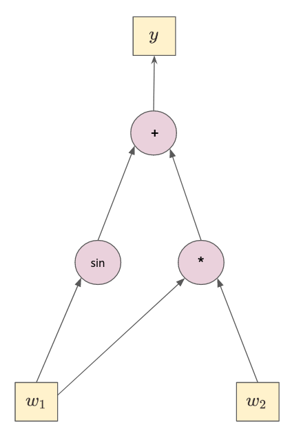
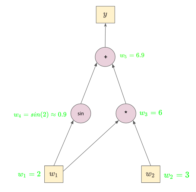
- Let's consider the following example:
$$
\boxed{
\begin{align*}
w_1 &= x_1 = 2
\\
w_2 &= x_2 = 3
\\
w_3 &= w_1w_2
\\
w_4 &= sin(w_1)
\\
w_5 &= w_3 + w_4 = y
\end{align*}
}
$$
- It can be represented as a **computational graph**.
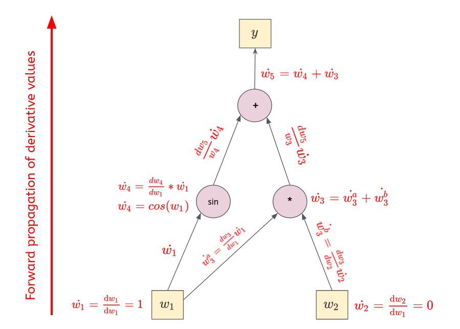
- Since $y$ depends on $w_1$ and $w_2$, its derivative will depend on $w_1$ and $w_2$ too. Thus, we have to perform 2 chain rules: $\frac{\mathrm{d} y}{\mathrm{d} w_1}$ and $\frac{\mathrm{d} y}{\mathrm{d} w_2}$.
- $\boxed{\text{For } \frac{\mathrm{d} y}{\mathrm{d} w_1}:}$
- Thus,
$$
\boxed{
\begin{align*}
\frac{\mathrm{d} y}{\mathrm{d} w_1} &= \dot{w_4} + \dot{w_3}
\\
&= cos(2)*1 + (1*3 + 2*0)
\\
&\approx 2.58
\end{align*}
}
$$
---
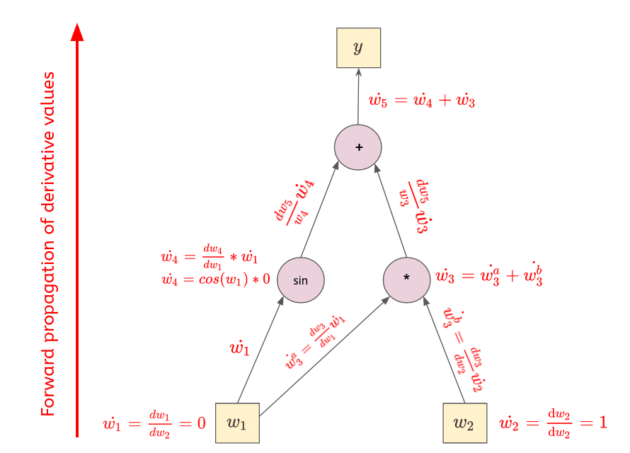
- $\boxed{\text{For } \frac{\mathrm{d} y}{\mathrm{d} w_2}:}$
- Thus,
$$
\boxed{
\begin{align*}
\frac{\mathrm{d} y}{\mathrm{d} w_2} &= \dot{w_4} + \dot{w_3}
\\
&= cos(2)*0 + (0*3 + 2*1)
\\
&\approx 2
\end{align*}
}
$$
---
- Setting $\dot{w_1}$ and $\dot{w_2}$ to $\{0, 1\}$ is called **seeding**.
- ==Forward AD is more efficient than Reverse AD for functions $f : \mathbb{R}^n \rightarrow \mathbb{R}^m$ with $m \gg n$ **(more outputs than inputs)** as only $n$ sweeps are necessary compared to $m$ sweeps for Reverse AD.==
### 2) Reverse automatic differentiation
- Reverse automatic differentiation is pretty much like Forward AD but this time, we traverse the chain rule from **left to right**. That is, according to our simple composition function, we first compute $\frac{\mathrm{d} y}{\mathrm{d} w_2}$ and then $\frac{\mathrm{d} w_2}{\mathrm{d} w_1}$ and finally $\frac{\mathrm{d} w_1}{\mathrm{d} x}$.
- Here is the recursive relation:
$$\boxed{\frac{\mathrm{d} y}{\mathrm{d} w_i} = \frac{\mathrm{d} y}{\mathrm{d} w_{i+1}} \frac{\mathrm{d} w_{i+1}}{\mathrm{d} w_{i}}}$$
- More precisely, we compute the derivative starting from the **outside to the inside**:
$$\boxed{\frac{\mathrm{d} y}{\mathrm{d} x} = \frac{\mathrm{d} y}{\mathrm{d} w_{i+1}} \frac{\mathrm{d} w_{i+1}}{\mathrm{d} x} = \left(\frac{\mathrm{d} y}{\mathrm{d} w_{i+2}} \frac{\mathrm{d} w_{i+2}}{\mathrm{d} w_{i+1}}\right)\frac{\mathrm{d} w_{i+1}}{\mathrm{d} x} = \left( \left(\frac{\mathrm{d} y}{\mathrm{d} w_{i+3}} \frac{\mathrm{d} w_{i+3}}{\mathrm{d} w_{i+2}}\right) \frac{\mathrm{d} w_{i+2}}{\mathrm{d} w_{i+1}}\right) \frac{\mathrm{d} w_{i+1}}{\mathrm{d} x} = ...}$$
- Let's consider the following example:
$$
\boxed{
\begin{align*}
w_1 &= x_1 = 2
\\
w_2 &= x_2 = 3
\\
w_3 &= w_1w_2
\\
w_4 &= sin(w_1)
\\
w_5 &= w_3 + w_4 = y
\end{align*}
}
$$
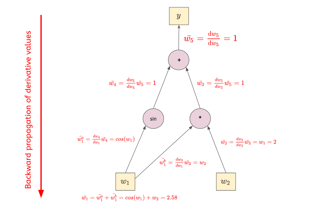
- It can be represented as a **computational graph**.
- The **reverse automatic differentiation** is divided into 2 parts:
- A **forward pass** to store intermediate values, needed during the backward pass.
- A **backward pass** to compute the derivatives.
---
### ☰ Forward pass
- We simply compute the value of each node. They will be used during the backward pass to compute the derivatives.
### ☰ Backward pass
- Using the previous recursive formula, we start from the output to the inputs.
- Thus,
$$\boxed{
\begin{align*}
\frac{\mathrm{d} y}{\mathrm{d} w_1} &= \bar{w_1} = cos(2) + 3 \approx 2.58
\\
\frac{\mathrm{d} y}{\mathrm{d} w_2} &= \bar{w_2} = 2
\end{align*}
}$$
---
- ==Reverse AD is more efficient than Forward AD for functions $f : \mathbb{R}^n \rightarrow \mathbb{R}^m$ with $m \ll n$ **(less outputs than inputs)** as only $m$ sweeps are necessary, compared to $n$ sweeps for Forward AD.==
## III) Implementation
- There are 2 ways to implement an autodiff:
- **source-to-source transformation** (hard):
- Uses a compiler to convert source code with mathematical expressions to source code with automatic differentiation expressions.
- **operator overloading** (easy):
- Users-defined data types and the operator overloading features of a language are used to implement automatic differentiation.
- Moreover, we usually have **less outputs than inputs in a neural network scenario**.
- Therefore, it is more efficient to implement the **Reverse AD** over the **Forward AD** mode.
- Our implementation revolves around the class `Node` which is defined below with its main components:
```python
class Node:
def __init__(self, data, requires_grad=True, children=[]):
pass
def zero_grad(self):
pass
def backward(self, grad=None):
pass
# Operators.
def __add__(self, other):
# built-in python operators.
pass
def matmul(self, other):
# custom operators.
pass
... # More operators.
# Functions.
def sin(self):
pass
... # More functions.
```
- Let's go through each method.
---
### 1) \_\_init\_\_() method
```python=
def __init__(self, data, requires_grad=True, children=[]):
self.data = data if isinstance(data, np.ndarray) else np.array(data)
self.requires_grad = requires_grad
self.children = children
self.grad = None
if self.requires_grad:
self.zero_grad()
# Stores function.
self._compute_derivatives = lambda: None
def zero_grad(self):
self.grad = Node(np.zeros_like(self.data, dtype=np.float64), requires_grad=False)
```
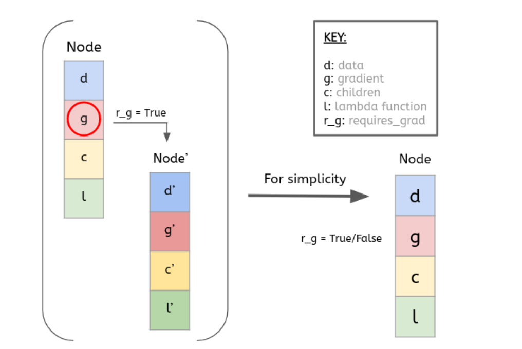
- The **\_\_init\_\_()** method has the following arguments:
- `data`: a scalar/tensor value.
- `requires_grad`: a boolean that tells us if we want to keep track of the gradient.
- `children`: a list to keep track of children.
- It has also other variables such as:
- `grad`: equal to 0-scalar/tensor (only if **requires_grad** is True) depending on `data` type.
- `_compute_derivatives`: lambda function, useful during **backward()** method (we will dive into it later on).
### 2) Operators & Functions
```python=
# Operators.
def __add__(self, other):
# Operator overloading.
op = Add(self, other)
out = op.forward_pass()
out._compute_derivatives = op.compute_derivatives
return out
def matmul(self, other):
# Custom matrix multiplication function.
op = Matmul(self, other)
out = op.forward_pass()
out._compute_derivatives = op.compute_derivatives
return out
# Functions.
def sin(self):
op = Sin(self)
out = op.forward_pass()
out._compute_derivatives = op.compute_derivatives
return out
# ------
# To make things clearer, I removed some line of codes.
# Check Yaae repository for full implementation.
class Add():
def __init__(self, node1, node2):
pass
def forward_pass(self):
# Compute value and store children.
pass
def compute_derivatives(self):
pass
class Matmul():
def __init__(self, node1, node2):
pass
def forward_pass(self):
# Compute value and store children.
pass
def compute_derivatives(self):
pass
class Sin():
def __init__(self, node1):
pass
def forward_pass(self):
# Compute value and store children.
pass
def compute_derivatives(self):
pass
```
- As you can see, the main strength of my implementation is that both **Operators and Functions follow the same structure**.
- Indeed, the code structure was designed in such a way it **explicitly reflects the Reverse AD mode logic** that is, ==first a forward pass and then a backward pass (to compute derivatives).==
- For each operator/function, the `forward_pass()` will create a new `Node` using the operator/function output with its children stored in `children`.
- And each `grad` will be a `Node` whose value is a 0-scalar/tensor depending on `data` type.
- We then compute the gradient using `compute_derivatives()` method of each operator/function classes.
- This method is then **stored in the lambda function `_compute_derivatives()` of each resulting nodes.**
- Notice that this method is not executed yet. We will see the reason later.
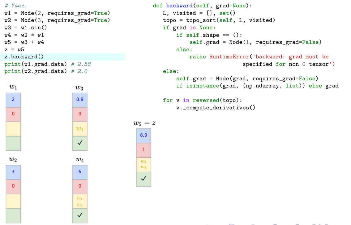
### 3) backward() method
```python=
def backward(self, grad=None):
L, visited = [], set()
topo = topo_sort(self, L, visited)
if grad is None:
if self.shape == ():
self.grad = Node(1, requires_grad=False)
else:
raise RuntimeError('backward: grad must be specified for non-0 tensor')
else:
self.grad = Node(grad, requires_grad=False) if isinstance(grad, (np.ndarray, list)) else grad
for v in reversed(topo):
v._compute_derivatives()
def topo_sort(v, L, visited):
"""
Returns list of all of the children in the graph in topological order.
Parameters:
- v: last node in the graph.
- L: list of all of the children in the graph in topological order (empty at the beginning).
- visited: set of visited children.
"""
if v not in visited:
visited.add(v)
for child in v.children:
topo_sort(child, L, visited)
L.append(v)
return L
```
- In the **backward()** method, we need to propagate the gradient from the output to the input as done in the previous example.
- To do so, we have to:
- Set `grad` of the output to 1.
- Perform a **topological sort**.
- Use the `_compute_derivatives()` lambda function which store the gradients of each node.
- A **topological sort** is performed for problems where some objects are ordered in a particular way.
- A typical example would be a set of tasks where certain tasks must be executed after other ones. Such example can be represented by a **Directed Acyclic Graph (DAG)** which is exactly the graph we designed.
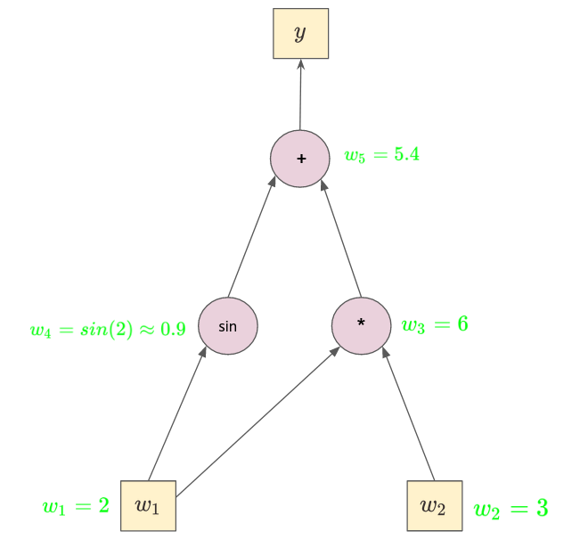 Figure: A computational graph (DAG)
- On top of that, order matters here (since we are working with chain rules). Hence, we want the node $w_5$ to propagate the gradient first to node $w_3$ and $w_4$.
- Now that we know a **topological sort** is needed, let's perform one. For the above DAG, the topological sort will output us `topo = [node_w1, node_w2, node_w3, node_w4, node_w5]`.
- We then reverse `topo` and call for each node in `topo` the `_compute_derivatives()` method which is a ==**lambda function** containing the node derivative computations, in charge of propagating the gradient through the DAG.==
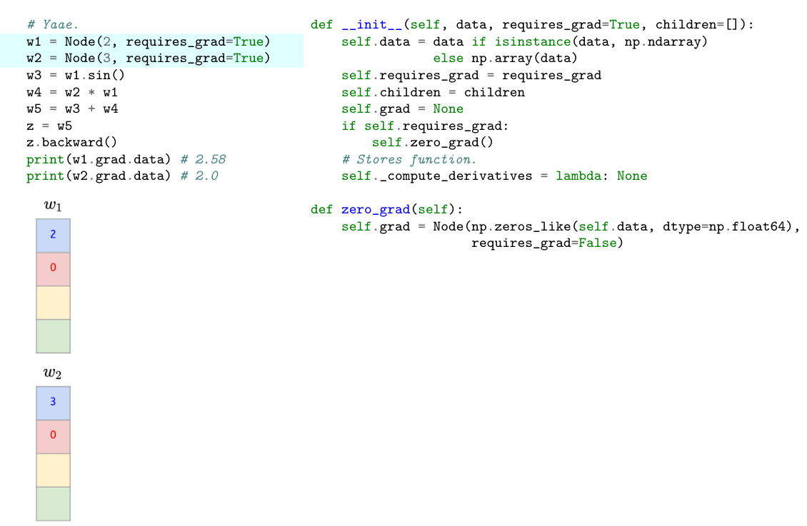
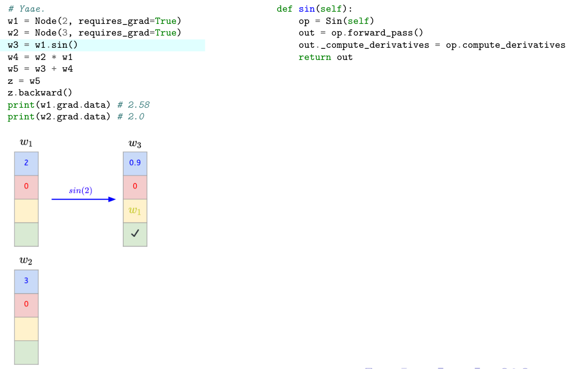
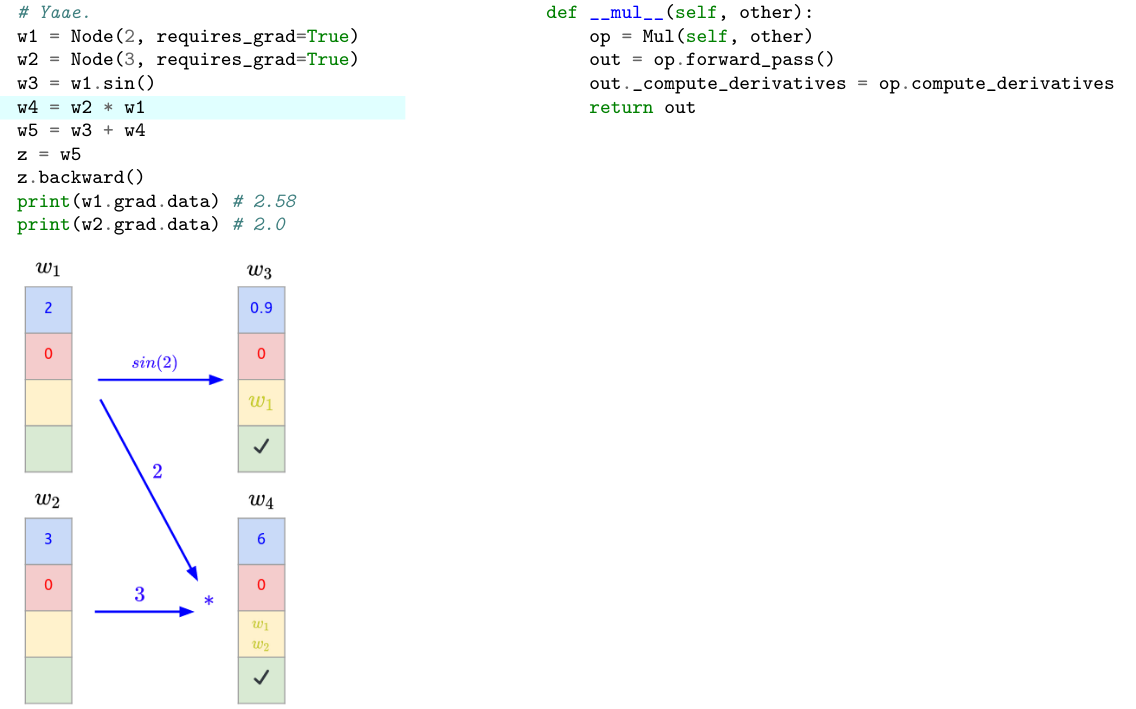
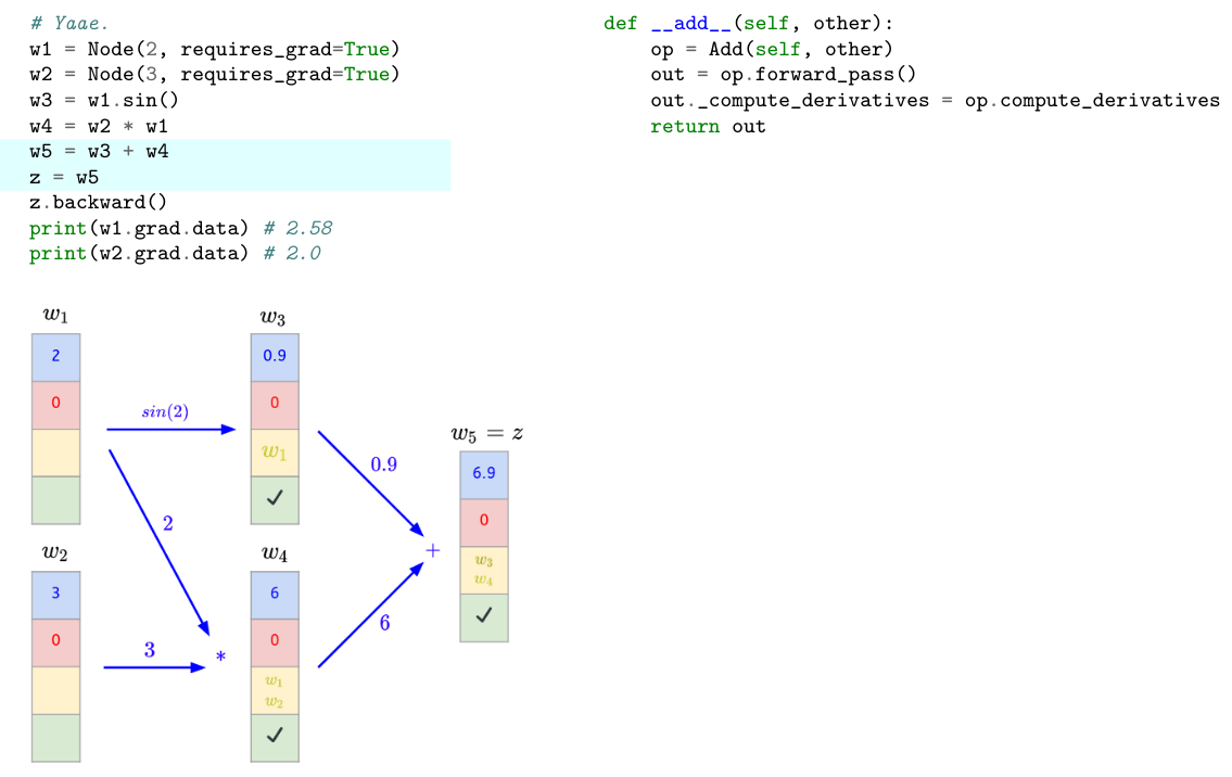
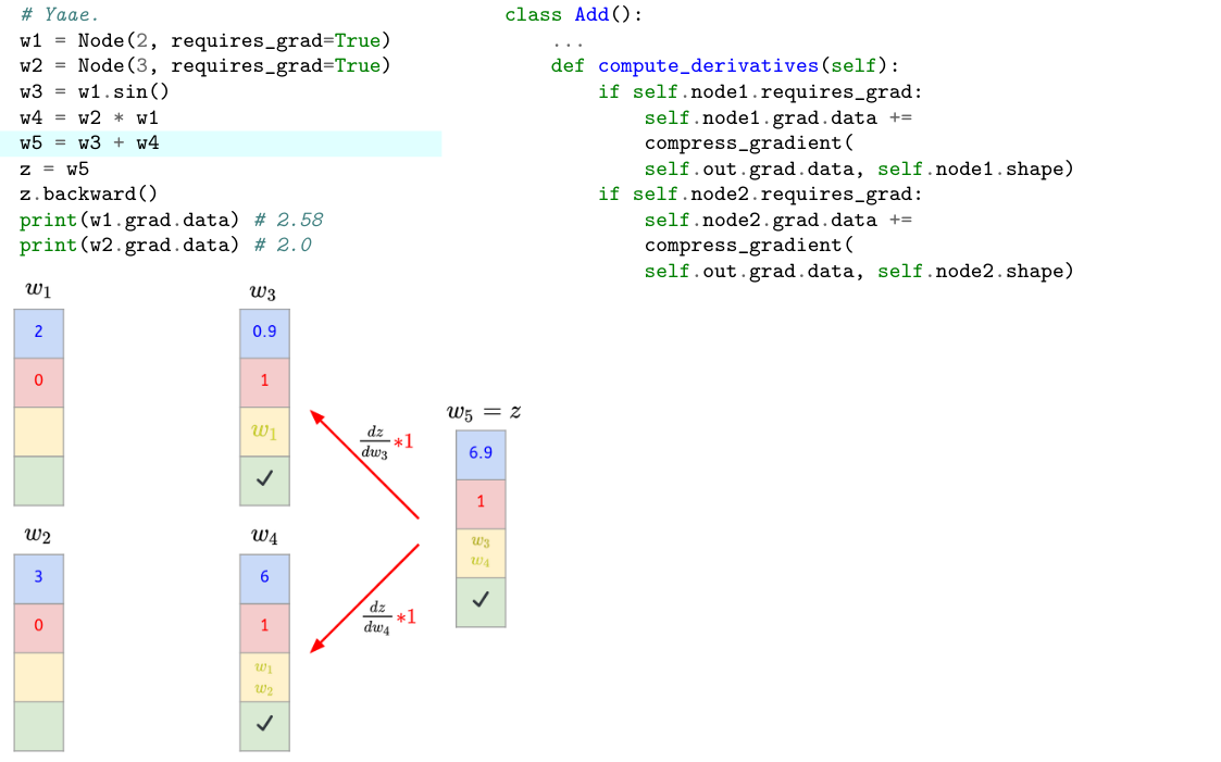
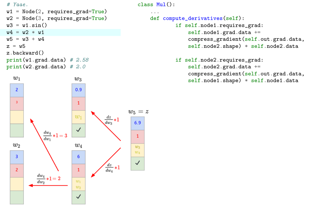
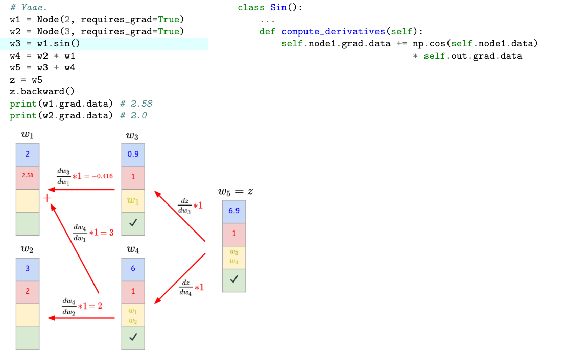
## IV) Application
- Let’s write down our previous example using Yaae and analyze itstep by step.
```python
# Yaae.
w1 = Node(2, requires_grad=True)
w2 = Node(3, requires_grad=True)
w3 = w2 * w1
w4 = w1.sin()
w5 = w3 + w4
z = w5
z.backward()
print(w1.grad.data) # 2.5838531634528574 ≈ 2.58
print(w2.grad.data) # 2.0
```
- Let's first define the following:
- In the following, the lambda function `l` will contain a check symbol to express that `l` is no more empty.
- It seems to work properly ! Since [Yaae](https://github.com/3outeille/Yaae) also supports tensors operations, we can easily build a small neural network library on top of it and workout some simple regression/classification problems !
- Here are the result from [demo_regression.ipynb](https://github.com/3outeille/Yaae/blob/master/src/example/demo_regression.ipynb) and [demo_classification.ipynb](https://github.com/3outeille/Yaae/blob/master/src/example/demo_classification.ipynb) files which can be found in the [repository example folder](https://github.com/3outeille/Yaae).
- Still skeptical ? We can even go further by writing our own [GAN](https://github.com/3outeille/GANumpy).