<small>(2016)Quadratic adaptive algorithm for solving cardiac action potential models</small>
===
<!-- .slide: data-background="#1A237E" -->
<small>
國立成功大學數學系
陳旻宏
2016/11/23
</small>
<small>Special Program in Applied Mathematics and Applied Mechanics,
CASTS, NTU</small>
[2019version](https://hackmd.io/SSQDZPkvQd6LYH2OTa1BZg)
---
## 研究團隊:
* 成功大學
* 電機系 羅錦興特聘教授(中山大學醫學科技研究所合聘)
* 數學系 陳旻宏副教授
* 中山大學
* 醫學科技研究所 陳志杰助理教授 (分子模擬)
* 高雄醫學大學附設醫院
* 工務室 陳博源博士
* 心臟內科 李香君 醫師/博士
* 陽明大學附設醫院 蘭陽院區
* 心臟內科 陳偉華 醫師/博士
----
## Outline
* Introduction
* Cardiac cell models
* Multidimensional Model
* Numerical Methods
* Numerical Results
* Conclusions
---
## Introduction
----
### Hodgkin and Huxley (HH) model
<p align="left"><small>Alan Hodgkin and Andrew Huxley described the model in 1952 to explain the ionic mechanisms underlying the initiation and propagation of action potentials in the squid giant axon (up to 1 mm in diameter).</small></p>
<!---They received the 1963 Nobel Prize in Physiology or Medicine for this work.
--->
{%youtube omXS1bjYLMI %}
https://www.ncbi.nlm.nih.gov/pmc/articles/PMC3424716/
----
#### Action potentials in Nerve Membranes
<p align="left"><small>When the action potential sweeps by the electrodes, the membrane is seen to depolarize (become more positive), overshoot the zero line, and then repolarize (return to rest)</small></p>

<p align="left"><small>Time course of membrane potential changes recorded with microelectrodes at two points in a squid giant axon stimulated by an electric shock</small></p>
----
### Hodgkin and Huxley (HH) model

----
* <small>The lipid bilayer: capacitance (Cm).</small>
* <small>Voltage-gated ion channels: electrical conductances</small>
* <small>The electrochemical gradients: voltage sources (En) </small>
* <small>ion pumps are represented by current sources (Ip).</small>
* <small>The membrane potential is denoted by $V_m$.</small>
* <small>Mathematically, the current flowing through the lipid bilayer is written as</small>
$\small I_{c}=C_{m} \frac{d}{dt} V_m$
* <small>the current through a given ion channel is the product </small>
$\small I_{i}={g_{n}}(V_{m}-V_{i})$
<small>where $V_{i}$ is the reversal potential of the i-th ion channel. Thus, for a cell with sodium and potassium channels, the total current through the membrane is given by: </small>
$\small I=C_{m} \frac{d V_m}{dt}+ g_{K}(V_m-V_K)+g_{Na}(V_m-V_{Na})+g_l(V_m-V_l)$
<small>$V_K$ and $V_{Na}$ are the potassium (鉀) and sodium (鈉) reversal potentials </small>
----

$\small I=C_{m} \frac{d V_m}{dt}+ g_{K}(V_m-V_K)+g_{Na}(V_m-V_{Na})+g_l(V_m-V_l)$
<small>$V_K$ and $V_{Na}$ are the potassium (鉀) and sodium (鈉) reversal potentials </small>
----
### 心跳週期
<small>
每個週期的開始都由竇房結(Sinoatrial node,簡稱S-A node)的自發性動作電位所引發。竇房結位於右心房後壁,能自主性產生頻率約為每分鐘70個的動作電位(action potential),因此做為整個心臟的節律點(pacemaker)。引發心臟收縮最初的動作電位即由此產生,並迅速地傳向左、右心房(atrial),然後經由房室結 (Atrioventricular node,簡稱A-V node)和希氏束(bundle of His)傳入心室。動作電位經過房室結後,經由左、右房室束分支(Left and Right bundle branch)以及柏金氏纖維(Purkinje fibers)傳遍左、右心室(ventricula)。
</small>

<!---柏金氏纖維由房室結開始,經過希氏束進入心室。因為它的心肌纖維非常粗大(直徑:35~40μm),比正常的心肌纖維(心室之心肌細胞直徑:10~25μm)還要粗,故其傳導神經衝動的速率非常地快,可達4.0m/s。這樣的特性使得心臟中的神經衝動能快速地傳遍整個心室系統。
--->
----
### Normal ECG

<small>
The action potentials from an atrial (green curve) and a ventricular (心室) fibre (blue curve) are shown above. – To the right is shown the direction of propagating waves in the frontal plane and their relation to the ECG waves.
http://www.zuniv.net/physiology/book/chapter11.html
</small>
----
### ECG and membrane potential
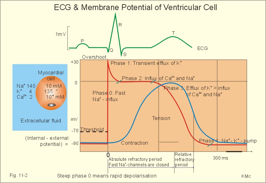
<small>
Recordings of ECG (above), intracellular membrane potential (red curve) and contraction (blue curve) of one heart cycle in a ventricular fibre
</small>
----
### Modeling cardiac action potentials
The cell membrane potential or voltage V then follows an ordinary differential equation
$dV/dt=−I_{ion}/C_m$,
where $I_{ion}$ is the sum of all transmembrane currents and $Cm$ is the membrane capacitance.
The negative sign is necessary because, by convention, inward currents are negative and outward currents are positive, so that a depolarizing inward current is negative but nonetheless increases the membrane potential.
----
### Modeling transmembrane currents
<small>
Action potentials are produced as a result of ionic currents that pass across the cell membrane, producing a net depolarization or repolarization of the membrane. The currents are produced by the movement of individual ions across the membrane through ion channels.</small>

----
### Modeling transmembrane currents
The most general form of a transmembrane current $I_Y$ permeable to ion Y is simply
$I_Y=g_Y(V−V_Y)$,
where $g_Y$ is a conductance term, $V$ is the membrane potential or voltage, and $V_Y$ is the Nernst potential (reversal potential) for ion species $Y$.
(The Nernst potential is the potential at which the electrical and chemical gradients across the membrane are balanced for that ion species and produce no movement of ions.
----
#### Gates
In practice, many cardiac ion channels are “gated” in a voltage-sensitive manner, so that the channels open and close in response to the membrane potential. Often these gates are represented using the Hodgkin-Huxley formalism.
The most common formulation for a gating variable $s$ is
$ds/dt=(s_{\infty}−s)/(\tau_s)$,
where $s_{\infty}$ is the voltage-dependent steady-state value of the gate and $\tau_s$ is the voltage-dependent time constant of the gate.
----
#### Markov chains

<small>
An alternative representation of gating can be achieved through Markov chains. In this case, each ion channel is represented by n discrete states representing various configurations of the channel, along with the rates at which transitions can occur from one state to another (these rates may be zero if it is not possible for the channel to switch directly between two given states).
</small>
----
#### Active Transport: pumps and exchangers
<small>
Along with ion channels, pumps and exchangers also transport ions across the membrane, in this case using active processes rather than simple diffusion. One of the most important of these is the Na+/Ca2+ exchanger, which under normal circumstances operates primarily to extrude Ca2+ ions from the cytoplasm by exchanging one Ca2+ ion for three Na+ ions, but which also operates in the reverse mode to extrude Na+ ions regularly following the rapid influx of Na+ ions through the fast Na+ channels but also abnormally in various pathophysiological states. Also important is the Na+/K+ pump, which extrudes Na+ that enters the cell from the fast Na+ channels by transporting three Na+ ions outside the cell and two K+ ions inside. Formulations for these currents follow similar principles but along with voltage must account for intracellular and extracellular concentrations of the relevant ions.</small>
----
### Modeling intracellular ion concentrations and processes
<small>The most common intracellular ion concentrations tracked in cardiac models are calcium, sodium, potassium, and occasionally chloride. The calcium concentration, in particular, is quite important, as it is the trigger for the cell to contract, and most models developed since 1977 include at least some basic intracellular calcium dynamics.
The intracellular sodium and potassium concentrations are more straightforward to represent and are updated simply in proportion to the sum of the transmembrane currents involving each ion (with appropriate weighting for the number of ions involved in pump and exchanger currents).</small>
----
#### sarcoplasmic reticulum (SR)
<small>Intracellular calcium models attempt to reproduce, at some level, the intricate dynamics of calcium within the cell. An increased level of intracellular calcium initiates the process of cell contraction, and cardiac cells whose primary function is to contract (the working ventricular myocytes) have specialized structures that facilitate this process. Calcium is stored internally in a structure called the sarcoplasmic reticulum (SR) . A relatively small influx of calcium through L-type calcium channels in the membrane triggers a comparatively large release of calcium from the internal store that increases the concentration of calcium in the cytosol by approximately a factor of ten. The calcium released binds to other compounds in the cell, which initiates the process of contraction.
Detailed models of calcium handling incorporate these different processes by including the channel through which calcium is released from the SR, ion diffusion within the SR, and reuptake of calcium back into the SR. More recently, some models also include a separate intracellular calcium concentration for the region near the L-type calcium channels, as these channels are predominantly located in a specific area with SR release channels located nearby, and it is hypothesized that a locally increased concentration is sensed in this region before the effects of diffusion equalize the calcium concentration throughout the cell.
Other more detailed ion handling can include buffering of different ions and ion diffusion throughout different parts of the cell.</small>
----
### [Cardiac action potential](https://en.wikipedia.org/wiki/Cardiac_action_potential)

---
## cardiac cell models
* Simplified Models
* FitzHugh-Nagumo (FHN) model for one cell (nerve)
* Karma model for one cell (generic cardiac)
* Ionic Models (Neuron)
* Hodgkin-Huxley model (Axon nerve, 1952)
### Heart Models
[Scholarpedia: Cardiac Cells](http://www.scholarpedia.org/article/Models_of_cardiac_cell)
----
### The Luo-Rudy guinea pig ventricular (LR91) model (8 variables)

[16] C.H. Luo, Y. Rudy, A Model of the Ventricular Cardiac Action-Potential - Depolarization, Repolarization, and Their Interaction, Circ. Res. 68 (1991) 1501-1526.
----
### The Luo-Rudy dynamic (LRd) model of the ventricular myocyte (15 variables)

----
### The O’Hara-Rudy ventricular myocyte dynamic model (2011)

----
<small>
O’Hara et al. constructed their model based on undiseased human heart data [17]. They replaced the L-type Ca2+ current, K+ currents, and Na+ /Ca2+ exchange in existing models. The ORd model enables us to simulate the three type epicardium cardiomyocyte (the epicardium, mid-myocardium and endocardium) electrophysiology by modify various ion channels parameters according to their electrophysiological characteristics.</small>
<small>
[17] T. O'Hara, L. Virág, A. Varró, Y. Rudy, Simulation of the Undiseased Human Cardiac Ventricular Action Potential: Model Formulation and Experimental Validation, PLoS Comput. Biol. 7 (2011) </small>
----
### The Markov IKs model

<small>
The Markov IKs model consists of two open states, O1 and O2, and 15 close states, C1 to C15.</small>
<small>
[24] J. Silva, Y. Rudy, Subunit interaction determines IKs participation in cardiac repolarization and repolarization reserve, Circulation 112 (2005) 1384-91.</small>
----
### Markov sodium channel model

----
<small> The wild-type channel model consists of three closed states (C3, C2, and C1), a conducting open state (O), and fast and slow inactivation states (IF and IS). The channel is very sensitive, and small time steps are required to stabilize the numerical simulation.
</small>

<small>
C. Clancy and Y. Rudy, Linking a genetic defect to its cellular phenotype in a cardiac arrhythmia. Nature. 400(1999). 566-569. </small>
---
## Multidimensional Model

<small>
* [thevirtualheart.org](https://thevirtualheart.org/)
* [Ventricular Tachycardia:心室跳動過速](https://en.wikipedia.org/wiki/Ventricular_tachycardia)
* [Ventricular Fibrillation: 心室顫動](https://zh.wikipedia.org/wiki/%E5%BF%83%E5%AE%A4%E9%A1%AB%E5%8B%95)
</small>
----
### Mono-domain model
Reaction-diffusion-like equation:
$\frac{\partial}{\partial t} V=−I_{ion}/C +\nabla \cdot (D\nabla V)$ (Eq.9)
Cell model (Ordinary differential equation):
$\frac{\partial}{\partial t} Y_i =\alpha_i (1−Y_i)−\beta_i Y_i$ (Eq.10)
$\frac{\partial}{\partial t} Z_i=f_i (1_{Z_i}, V,Z_i )$ (Eq.11)

<!---
#### Excitable Media:
An excitable medium is a dynamical system distributed continuously in space, each elementary segment of which possesses the property of excitability. Neighboring segments of an excitable medium interact with each other by diffusion-like local transport processes. In an excitable medium it is possible for excitation to be passed from one segment to another by means of local coupling. Thus, an excitable medium is able to support propagation of undamped solitary excitation waves, as well as wave trains.
http://www.scholarpedia.org/article/Excitable_media
--->
----
#### Propagating plane wave on a slab, with spatial and temporal recording.

----
##### Timing is everything:
| 描述 | Simulation |
|:--- |:----:|
| <small>Target pattern from a late premature stimulus following a plane wave </small>|  |
<small>Disappearing early premature stimulus following a plane wave. </small>||
<small>Counter-rotating spiral waves induced by a carefully timed premature stimulus following a plane wave.</small>|
----
### [Experimental Movies](http://thevirtualheart.org/movies/experimental.html#optical)
<small>Propagating wave from a point stimulus </small>

|<small>Spiral wave (Reentry)</small>|<small>Spiral wave (Reentry)</small>|
|:---:|:---:|
|
----
|<small>Spiral wave (Reentry)</small>|<small>Spiral wave (Reentry)</small>|
|:---:|:---:|
|
|<small>Spiral wave breakup </small>|<small> More complex activity </small>|
|:---:|:---:|
|
[Optical mapping (Tissue)](http://thevirtualheart.org/movies/experimental.html#optical)
---
## Numerical Methods
----
### Rush-Larsen method
* The gating variables as functions of the membrane potential and time are written as
$du_i/dt = \alpha_{u_i}(1-u_i)- \beta_{u_i} u_i , i = 1,2,⋯,n$ (1)
where $\alpha_{u_i}(V)$ and $\beta_{u_i}(V)$ are voltage-dependent gating variables.
* If the $\alpha_{u_i}(V)$ and $\beta_{u_i}(V)$ are assumed to be constant,
$u_i(t)= u_i(\infty)-[u_i(\infty)-u_i(0)]\cdot \exp{( -t/\tau_i)}$ (2)
where $\tau_i =1/(\alpha_{u_i}+\beta_{u_i})$, $u_i(\infty) = (\alpha_{u_i})/(\alpha_{u_i}+\beta_{u_i})$
----
### Hybrid method
<p>
<small>
The so-called Hybrid method was based on the variable time step of the RL method proposed by Victorri B. et al. [6].
</small>
</p>
The Hybrid method procedure is operated with:
* If $\Delta V \le \Delta V_{min}$ , then $\Delta t = \Delta V_{max} / (dV/dt)$ (3)
* If $\Delta V \ge \Delta V_{max}$ , then $\Delta t = \Delta V_{min}/(dV/dt)$ (4)
* If $\Delta V_{max} > \Delta V > \Delta V_{min}$ , then $\Delta t = \Delta V$ (5)
* If $\Delta t \ge \Delta t_{max}$ , then $\Delta t = \Delta t_{max}$ (6)
<small>
where $\Delta V$ is the change in the membrane potential, $\Delta V_{min}$ is the lower bound, and $\Delta V_{max}$ is the upper bound.
</small>
* In the study, we consider the Hybrid method with voltage couplets ($\Delta V_{min}$ to $\Delta V_{max}$ ), 0.05-0.2 mV.
----
### Proposed CCL method
#### Second-order Taylor expansion: Eq(7)
$\small V(t_{n+1}) \cong V(t_n)+ V'(t_n)\dot (t_{n+1}- t_n) +V''(t_n)/2! \cdot (t_{n+1}- t_n)^2$
* Goal: $\small \Delta V \cong dV/dt\, \cdot \Delta t + 1/2 \cdot d^2 V/ dt^2 \cdot \Delta t^2$,
* $\small d^2 V/dt^2 \cong (V'(t_n)-V'(t_{n-1}))/ \Delta t_n.$
#### New Time Step Size: Eq(9)
$\small \Delta t = (-dV/dt \pm \sqrt{(dV/dt)^2+2 \cdot d^2 V/dt^2 \cdot \Delta V})/(d^2 V/dt^2).$
#### Other features
* Extremum-locator (el): $\small \Delta t_Z = - (dV/dt)/(d^2 V/dt^2)$
* Time step restriction (tsr): $\small \Delta t_{n+1} \le 2 \Delta t_n$.
---
## Numerical Results
### [Cardiac action potential](https://en.wikipedia.org/wiki/Cardiac_action_potential)

----
### LR1 model (8 variables)
![]
----

----
### LR2-RV model

$APD_{90}$ of 500 beats of LR2-RV model generated by the Hybrid and CCL methods.
<small>APD: Action potential duration</small>
----
| CCL | Hybrid |
|:------:|:-----------:|
|  | 
----
| $I_{to}$ | $I_{Cal}$ |
|:------:|:-----------:|
|  | 
* <small>Ito: Transient Outward Current</small>
* <small>ICal: L-type Ca2 current</small>
----
Time-step size
| CCL | Hybrid |
|:------:|:-----------:|
|  | 
----
| Hybrid | CCL |
|:------:|:-----------:|
|  | 
----
| Hybrid | CCL |
|:------:|:-----------:|
|  | 
----
| Hybrid | CCL |
|:------:|:-----------:|
|  | 
----
### ORd with the human Markov $I_{K_s}$ model
| $0.001ms - 1 ms$ | $0.001ms - 0.1ms$ |
|:------:|:-----------:|
| | 
----
Zoom-in
| $0.001ms - 1 ms$ | $0.001ms - 0.1ms$ |
|:------:|:-----------:|
| | 
----
### 3.5 Courtemanche – Markov $I_{N_a}$ model
#### Membrane Potential
| CCL $0.001ms - 1 ms$ | Hybrid $0.001ms - 1ms$ |
|:------:|:-----------:|
| | 
----
#### $I_{Na}$
| CCL $0.001ms - 1 ms$ | Hybrid $0.001ms - 1ms$ |
|:------:|:-----------:|
| | 
----
#### dt
| CCL $0.001ms - 1 ms$ | Hybrid $0.001ms - 1ms$ |
|:------:|:-----------:|
| | 
----
#### Membrane Potential
| CCL $0.001-0.1ms$ | Hybrid $0.001 -0.1ms$ |
|:------:|:-----------:|
| | 
----
#### $I_{Na}$
| CCL $0.001 - 0.1 ms$ | Hybrid $0.001 - 0.1ms$ |
|:------:|:-----------:|
| | 
----
#### dt
| CCL $0.001 - 0.1 ms$ | Hybrid $0.001 - 0.1ms$ |
|:------:|:-----------:|
| | 
---
## Multidimensional Simulations

[reference]: https://thevirtualheart.org/
----
### Mono-domain model
<small>Reaction-diffusion-like equation:</small>
* $\small \frac{\partial}{\partial t} V=−I_{ion}/C+\nabla \cdot (D\nabla V)$
<small>Cell model (Ordinary differential equation):</small>
* $\small \frac{\partial}{\partial t} Y_i =\alpha_i (1−Y_i )−\beta_i Y_i$, $\small \frac{\partial}{\partial t} Z_i=f_i (I_{Z_i}, V,Z_i )$
#### Qu-Garfinkle (IEEE 1999)
* Equation: $\small dV/dt=(\Gamma_1+\Gamma_2 )V$
* $\small V(t+\Delta T)=e^{(\Gamma_1+\Gamma_2 )\Delta T} V(t)$
* $\small V(t+\Delta T)=e^{(\Gamma_2 \Delta T/2)} e^{(\Gamma_1 \Delta T)} e^{(\Gamma_2 \Delta T/2)} V(t)+o(\Delta t^3 )$
----
ORd 500x500
{%youtube RBC-p9CU-E0 %}
----
ORd 500x500
{%youtube H3jzryET_1Y %}
----
ORd 1000x1000
{%youtube js5f-h9Cn0s %}
----
No Blockage in $I_K$
{%youtube icoyykzdDOo %}
----
With Blockage in $I_K$
{%youtube 15i-HrKzZoA %}
---
## Conclusions
* The proposed method is more accurate than and as efficient as the Hybrid method, especially for the ORd model.
* The proposed method can properly adjust the time step size according to the change in the potential.
* The proposed method is more stable for stiff Markov chain-type ionic models.
* A protective zone is not required for our method in the upstroke region.
----
### Reference
[Scholarpedia: Cardiac Cells](http://www.scholarpedia.org/article/Models_of_cardiac_cell)
[CellML](http://www.cellml.org/)
[Rudy Lab](http://rudylab.wustl.edu/research/cell/index.html)
[ModelDB](https://senselab.med.yale.edu/modeldb/default.cshtml)
[thevirtualheart.org](http://thevirtualheart.org/)
http://highscope.ch.ntu.edu.tw/wordpress/?p=27705
---