# Time series ch.18 & ch.19

In the previous chapter, we learned the basics of forecasting and some modeling techniques.
However, we learned about models, not complete forecasting systems.

What follows is a subtle departure from the basics.
You'll learn about

• Why multi-step forecasting?
• Recursive strategy
• Direct strategy
• Joint strategy
• Hybrid strategies
• How to choose a multi-step forecasting strategy

우리는 이전 챕터에서 forecasting의 기본과 몇 가지의 모델링에 대한 기술들을 배웠습니다.
하지만 이는 완전한 forecasting system이 아닌 모델들에 대해서 배웠습니다.

이후에 다룰 내용들은 기본적인 내용들과 미묘하게 다른 부분들입니다.
아래와 같은 내용에 대해서 다룹니다.

• Why multi-step forecasting?
• Recursive strategy
• Direct strategy
• Joint strategy
• Hybrid strategies
• How to choose a multi-step forecasting strategy

## Why mulit-step forecasting?

Multi-step forecasting is the task of predicting the next $H$ time steps $y_{t+1} , ... , y_{t+H}$ for the time series $y_1 , .... , y_t \ \ \ \ where \ \ H > 1$.
We often see these applications in real life. For example, if you want to predict electricity usage in the summer, it's more useful to look at a week's or month's usage than an hour's usage.
If you can forecast usage over a longer period of time, you can use it to efficiently adjust your power production.

The utility of such multi-step forecasting has not received much attention.
This is because methods such as ARIMA and exponential smoothing existed, and these techniques can be made multi-step.
But with the advent of ML and deep learning, multi-step forecasting like this is starting to gain traction.

Another reason why multi-step forecasting is less popular is that it's harder than single-step forecasting. The more steps you have to estimate the future, the harder it is to make a prediction because of the interactions between each step.

That's why we use the following strategies

multi-step forecasting은 time series $y_1 , .... , y_t \ \ \ \ where \ \ H > 1$에 대해서 next $H$ time steps $y_{t+1} , ... , y_{t+H}$를 예측하는 일입니다.
실생활에서 이러한 응용들을 자주 쓰입니다. 예를 들면 여름의 전기 사용량을 예측한다고 할 때 한 시간의 전기 사용량 보다는 일주일 혹은 한달 정도의 전기 사용량이 조금더 쓸모 있을 것입니다.
긴 기간의 사용량을 예측을 할 수 있다면 이를 이용해서 전력 생산량을 효율적으로 조절 할 수 있을 것입니다.

이러한 다단계의 예측의 쓸모가 있더라도 주목을 받지 못했습니다.
ARIMA와 exponential smoothing와 같은 method들이 존재했기 때문입니다. 이러한 기법들은 multi-step을 만들 수 있기 때문입니다.
하지만 ML과 Deep Learning의 등장으로 이와 같은 multi-step forecasting이 주목을 받기 시작했습니다.

multi forecasting이 인기가 낮은 또 다른 이유는 single step forecasting보다 어렵기 때문입니다. 미래를 추정하는 단계가 많을수록 각 단계간의 상호작용 때문에 예측을 하기 어려워집니다.

그래서 다음과 같은 전략들을 사용합니다.


For the annotations we will use in this chapter, we define them as follows

$\mathbb{Y}$: $T$ time serts, $y_1 , ... y_t$, a time series with the same meaning as $T$ but with a time step ending at $t$.

$\boldsymbol{W}$ : function to generate a window with $k > 0$, a proxy used for input to various models.

$H$ :forecast horizon

이장에서 사용할 annotation에 대해서 다음과 같이 정의합니다.

$\mathbb{Y}$ : $T$ time serts, $y_1 , ... y_t$와 같은 의미이지만 time step이 $t$에서 끝나는 time series입니다.

$\boldsymbol{W}$ : $k > 0$인 window를 생성하는 함수 , 다양한 모델의 input에 사용하는 프록시입니다.

$H$ :forecast horizon

## Recursive strategy

The recursive strategy is the most intuitive and popular multi-step forecasting method.
You should know the following

Recursive strategy는 가장 직관적이고 인기 있는 multi-step forecasting 방법입니다.
다음과 같은 내용을 알야야 합니다.

• How is the training of the models done?
• How are the trained models used to generate forecasts?


#### Training regime

training works by predicting the very next step.
We create a window and train it using the window function $\boldsymbol{W}(\mathbb{Y}_t)$, as shown in the figure above. The model predicts $y_{t+1}$.
The loss function optimizes the params using the difference between $\hat{y_{t+1}}$ and $y_{t+1}$.

training은 바로 다음 step을 예측하는 방식으로 학습을 합니다.
위 그림에서와 같이 윈도우 함수를 $\boldsymbol{W}(\mathbb{Y}_t)$를 이용하여 윈도우를 만들고 이를 훈련합니다. 모델은 $y_{t+1}$을 예측합니다.
loss function은 $\hat{y_{t+1}}$ 와 $y_{t+1}$의 차이를 이용해서 params를 최적화 합니다.

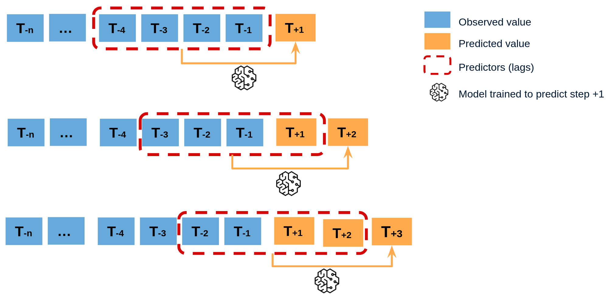
#### Forecasting regime

We've built our model to predict one-step-ahead. Let's use it to recursively predict $H$ timesteps.
We start by creating $\hat{y_{t+1}}$.
Use it to create a new window $\boldsymbol{W}(\mathbb{Y}_t : \hat{y_{t+1}})$ to predict $\hat{y_{t+2}}$.
Repeat this for $H$ sizes.

모델을 one-step-ahead를 prediction하도록 모델을 만들었습니다. 이를 이용해서 재귀적으로 $H$ timesteps 를 예측하도록 합니다.
우선 먼저 $\hat{y_{t+1}}$을 생성합니다.
이를 이용해서 새로운 window $\boldsymbol{W}(\mathbb{Y}_t : \hat{y_{t+1}})$ 을 생성해서 $\hat{y_{t+2}}$를 예측합니다.
이러한 방식을 $H$ 크기만큼 반복합니다.


This is how classical time series models (ARIMA , exponential smoothing models) work internally.

이러한 방식은 고전적인 시계열 모델(ARIMA , 지수 평활화 모델)에서 내부적으로 동작하는 방식입니다.

## Direct strategy

This strategy is also known as an independent strategy.
This is a popular approach for methods using ML.
It is a method that predicts each horizon independently.

이 방식은 independent strategy라고도 불리는 방식입니다.
이 방식은 ML을 이용한 방식에서 인기 있는 방식입니다.
각 horizon을 독립적으로 예측하는 방식입니다.


#### Training regime
For each horizon, you want to run each model separately to make predictions at different times.
There are two ways to implement this approach.

각각의 horizon에 대해서 각 모델을 개별적으로 각각의 다른 시간대로 예측하도록 예측을 합니다.
이 방식을 구현하는 방식은 2가지 방식이 있습니다.

• Shifting targets – Each model in the horizon is trained by shifting the target by that many
steps as the horizon we are training the model to forecast.

• Eliminating features – Each model in the horizon is trained by using only the features that are allowable to use according to the rules. For instance, when predicting $𝐻 = 2$, we can’t use lag 1 (because to predict $𝐻 = 2$, we will not have actuals for $𝐻 = 1$).

#### Forecasting regime

Forecasting is also straightforward. For each trained model, you just need to predict the values independently.

forecasting도 간단하게 할 수 있습니다. 훈련된 각 모델에 대해서 독립적으로 값들을 예측을 하면 됩니다.

## Joint strategy

The two models described above are multi input single output.
The way to change this to mutliple input , multiple output (MIMO) is the joint strategy.

앞서 설명한 두 모델은 multi input single output을 가지는 구조입니다.
이를 mutliple input , multiple output(MIMO)로 바꾸는 방식이 Joint strategy입니다.


#### Training regime
This approach trains one model to predict all horizons at once.

이 방식은 하나의 모델을 훈련하여 모든 horizon을 한번에 예측하는 방식입니다.

#### Forecasting regime
Since the model can predict all horizons, we can just make a prediction.
This approach is often used in DL models when the output H of the last layer is 1.

모델이 모든 horizon을 예측 할 수 있으므로 그냥 예측을 하면 됩니다.
이러한 방식은 DL model 중에서도 last layer의 output H 이 1인 경우에 주로 사용합니다.

## Hybrid strategies
The strategies described above are basic, and you can combine them to get even better performance. We'll cover just a few of the most common strategies.

위에서 설명한 strategies는 기본적인 strategies입니다. 이를 조합하면 더 좋은 성능을 보일 수 있을 것입니다. 대표적인 몇 가지의 strategies만 다뤄보겠습니다.

### DirRec Strategy
As the name implies, this method is a combination of direct and recursive.

이 방식은 이름에서도 유추할 수 있듯이 direct와 recursive을 합친 방법입니다.


#### Training regime

Similar to the direct strategy, DirRec requires $H$ models for each horizon. But it's a little different. In Direct, we were predicting one step ahead, and in Recurive, we were predicting by the size of H.
However, in DirRec, we train with $H = 2$, but the actual prediction is made with $H = 1$. A generalization of this is to train a separate model for each h for $h < H$, and then make a prediction on that.

direct strategy와 유사하게 DirRec방속 또한 각 horizon마다 $H$ 개의 모델이 필요합니다. 하지만 조금은 다릅니다. Direct에서는 한 단계 앞을 예측하고, Recurive에서는 H을 크기만큼을 예측을 했습니다.
하지만 DirRec에서는 $H = 2$로 훈련을 하지만 실제 예측은 $H = 1$로 예측을 합니다. 이를 일반화 하면 $h < H$에 대하여 각 h마다 각각의 모델을 훈련후 이를 예측을 합니다.

#### Forecasting regime

Similar to training, but using the $H$th trained model for prediction. You'll make predictions in the same way as recursive.

학습과 유사하지만 $H$ 번째 훈련된 모델을 예측을 사용합니다. recursive와 같은 방식으로 예측을 하게 됩니다.

### Iterative block-wise direct strategy

This method makes iterative predictions in blocks to compensate for the fact that the Direct method trains each model $H$, which makes it difficult to make long-term predictions.

이 방식은 Direct 방식의 각각의 모델 $H$를 학습 시키므로 인해서 이를 장기 예측을 하기 힘들다는 단점을 보완하기 위해서 block 단위의 반복적인 예측을 합니다.


#### Training regime
In IBD, we split the forecast horizon $H$ into $R$ blocks and $L$ legnths so that $H = L \times R$. Instead of training $H$ models, we train $L$ models.

IBD에서는 forecast horizon $H$를 $R$ block과 $L$ legnth로 분리 해서 $H = L \times R$이 되도록 합니다. $H$개의 모델을 훈련하는 대신에 $L$개의 모델을 훈련합니다.

#### Forecasting regime

Predict frist $L$ time steps using $L$ trained models.
Predict $T+1 \ to \ T+L$. Take this prediction horizon as input again and predict $\boldsymbol{W}(\mathbb{Y}_T : \mathbb{Y}_{T+L})$ as input again. Repeat this $R-1$ times.

학습한 $L$개의 모델을 이용해서 frist $L$ time steps를 예측합니다.
$T+1 \ to \ T+L$ 만큼을 예측합니다. 이 예측 horizon을 다시 input으로 해서 $\boldsymbol{W}(\mathbb{Y}_T : \mathbb{Y}_{T+L})$을 input으로 다시 예측을 합니다. 이와 같은 작업을 $R-1$회 반복을 합니다.

### Rectify strategy
This is another way to combine a direct strategy with a recursive strategy.
It's a kind of stacking approach.

이 방식은 direct strategy와 recursive strategy을 합치는 또 다른 방식입니다.
일종의 stacking 방식입니다.


#### Training regime
The training is done in two steps Generate timesteps up to all $H$ using the Recurvie model. Let's call them $\widetilde{\mathbb{Y}_{t+H}}$. Put $\widetilde{\mathbb{Y}_{t+H}}$ back into the direct model.

학습은 두 단계로 이루어 집니다. Recurvie 모델을 이용해서 모든 $H$ 까지의 timestep을 생성합니다. $\widetilde{\mathbb{Y}_{t+H}}$라고 합니다. $\widetilde{\mathbb{Y}_{t+H}}$를 다시 direct 모델에 넣습니다.

#### Forecasting regime
To create inputs similar to train, but in a direct way, the Rec model is processed in parallel to create inputs and use them to make predictions.

train과 유사하지만 direct 방식의 input을 만들기 위해서 Rec model을 병렬적으로 처리후에 input을 만들고 이를 이용해서 예측을 합니다.

### RecJoint

This method is a mashup of the recursive and joint methods. However, this model can also be used with a single output.

이 방식은 recurive와 joint 방식의 mashup 방식입니다. 하지만 이모델은 single output도 사용할 수 있습니다.


#### Training regime

If the recursive made a prediction at $t+2$ with input at $t+1$, this method trains over the entire horizon and optimizes the output.

recurive에서 $t+1$에서의 입력으로 $t+2$를 예측을 했다면 이 방식은 전체 horizon에 대해서 훈련을 합니다. 이때 나온 output을 최적화 합니다.

#### Forecasting regime
Predict is also very similar to recursive.

예측도 recurive와 매우 유사합니다.

## How to choose a multi-step forecasting strategy?


• Engineering complexity: Recursive, Joint, RecJoint << IBD << Direct, DirRec << Rectify

• Training time: Recursive << Joint (typically $T_{mo}$ > $T_{so}$) << RecJoint << IBD << Direct, DirRec << Rectify

• Inference time: Joint << Direct, Recursive, DirRec, IBD, RecJoint << Rectify

# ch.18 Evaluating Forecasts – Forecast Metrics

We have been using a few metrics throughout the book and it is now time to get down into the details to understand those metrics, when to use them, and when to not use some metrics. We will also elucidate a few aspects of these metrics experimentally.

In this chapter, we will be covering these main topics:

• Taxonomy of forecast error measures
• Investigating the error measures
• Experimental study of the error measures
• Guidelines for choosing a metric

## Taxonomy of forecast error measures

In general regression, metrics such as MSE and MAE are not used, but in time series, there are many metrics.
The important factors of metrics in time series can be categorized into three main categories.

일반적인 regression에서는 MSE , MAE와 같은 metric은 줄 사용하지 않으나 time series에서는 수많은 metric이 있습니다.
time series의 metric의 중요한 factor는 크게 3가지로 구분할 수 있습니다.

• Temporal relevance: The temporal aspect of the prediction we make is an essential aspect of a forecasting paradigm. Metrics such as forecast bias and the tracking signal take this aspect into account.

• Aggregate metrics: In most business use cases, we would not be forecasting a single time series, but rather a set of time series, related or unrelated. In these situations, looking at the metrics
of individual time series becomes infeasible. Therefore, there should be metrics that capture the idiosyncrasies of this mix of time series.

• Over- or under-forecasting: Another key concept in time series forecasting is over- and under forecasting. In a traditional regression problem, we do not really worry whether the predictions are more than or less than expected, but in the forecasting paradigm, we must be careful about structural biases that always over- or under-forecast. This, when combined with the temporal aspect of time series, accumulates errors and leads to problems in downstream planning

앞서 설명한 factor들을 고려했을때 metric을 짜면 많은 metirc이 나옵니다. 이러한 metirc들을 분류 해보겠습니다.


Metrics can be broadly divided into intrinsic and extrinsic.

metric은 크게 intrinsic and extrinsic으로 나눌 수 있습니다.

* intrinsic metric은 생성된 forecasting과 이에 대응하는 actual값을 측정하는 방식입니다.
* extrinsic metric은 생성된 예측을 포함해서 외부 참조 혹은 벤치마크들을 확인해서 측정하는 방식입니다.

For ease of understanding, we define the following symbols
$y_t$: the actual value at time t
$\widehat{y_t}$: the predicted value of the modeldel at time t
$H$: forecast horizon
$m$ : indexed by $m$ of the $M$ time series
$e_t$ : $y_t - \widehat{y_t}$

이해를 쉽게 하기 위해서 다음과 같은 기호를 정의합니다.
$y_t$ : t 시점에서의 실제값
$\widehat{y_t}$ : t 시점에서의 모데델의 예측 값
$H$ : forecast horizon
$m$ : $M$ time series의 indexed by $m$
$e_t$ : $y_t - \widehat{y_t}$

## Intrinsic metrics
here are four major base errors – absolute error, squared error, percent error, and symmetric error

다양한 metric을 알아보기전에 기본 오차에 대해서 알아봅시다.







## Extrinsic metrics

### Relative

The big problem with Intrinsic metrics is that there are no benchmarks.
If we say MAPE is 5%, that might be a bad performance because we don't know how predictable this time series is.

$y_t^*$ : Benchmark predicted value
e_t^*$ : Benchmark error

There are two ways to set up your benchmarks

Intrinsic metrics은 벤치마크가 없다는 점이 큰 문제입니다.
만약에 MAPE가 5%라고하면 이 시계열이 얼마나 예측 가능한지 모르기 때문에 이는 좋지 않은 성능일 수도 있습니다.

$y_t^*$ : 벤치마크 예측값
$e_t^*$ : 벤치마크 에러

벤치마크를 설정하는 방식은 다음과 같이 2가지가 있습니다.

• Using errors from the benchmark forecast to scale the error of the forecast
• Using forecast measures from the benchmark forecast to scale the forecast measure of the forecast we are measuring




## Investigating the error measures

It's better to understand the properties of the underlying metirc than to know multiple metrics in order to compare how error behaves and what makes it good or bad.

error가 어떻게 동작하고, 어떤 점에서 좋은지 안 좋은지를 비교하기 위해서는 여러 metric을 알기 보다는 기본 metirc의 속성을 이해하는 것이 좋습니다.

### Loss curves and complementarity

이러한 모든 기본 오차는 예측과 실제 관측이라는 두 가지 요소에 따라 달라집니다. 한 가지를 수정하면 이러한 여러 지표의 이러한 여러 지표의 동작을 조사할 수 있습니다. 오류. 예상되는 것은 양쪽의 실제 관측값과의 편차 편차는 편향되지 않은 지표에서 똑같이 불이익을 받아야 하기 때문입니다. 우리는 예측과 실제 관측을 바꿀 수도 있으며, 이 경우에도 메트릭에 영향을 미치지 않아야 합니다. 노트북에서 손실 곡선과 상보 쌍을 정확히 이러한 실험을 수행했습니다.

All these base errors depend on two factors – forecasts and actual observations. We can examine the behavior of these several metrics if we fix one and alter the other in a symmetric range of potential errors. The expectation is that the metric will behave the same way on both sides because deviation from the actual observation on either side should be equally penalized in an unbiased metric. We can also swap the forecasts and actual observations and that also should not affect the metric. In the notebook, we did exactly these experiments – loss curves and complementary pairs.

#### error plot





### Bias towards over- or under-forecasting

Under- and over-forecast for several metrics.
몇 가지 지표에 대해서 under-forecasting과 over-forecasting이 되는지 알아봅니다.



To summarize the results

결과를 요약하면 다음과 같습니다.

• MAPE clearly favors the under-forecasted with a lower MAPE than the over-forecasted.
• WAPE, although based on percent error, managed to get over the problem by having explicit weighting. This may be counteracting the bias that percent error has.
• sMAPE, in its attempt to fix MAPE, does a worse job in the opposite direction. sMAPE highly favors over-forecasting.
• Metrics such as MAE and RMSE, which are based on absolute error and squared error respectively, don’t show any preference for either over- or under-forecasting.
• MASE and RMSSE (both using versions of scaled error) are also fine.
• MRAE, in spite of some asymmetry regarding the reference forecast, turns out to be unbiased from the over- and under-forecasting perspective.
• The relative measures with absolute and squared error bases (RelMAE and RelRMSE) also do not have any bias toward over- or under-forecasting.
• The relative measure of mean absolute percentage error, RelMAPE, carries MAPE’s bias toward under-forecasting.
We have investigated a few properties of different error measures and understood the basic properties of some of them. To further that understanding and move closer to helping us select the right measure for our problem, let’s do one more experiment using the London Smart Meters dataset we have been using through this book.

### Guidelines for choosing a metric

Now that you know the pros and cons of each metric, let's talk about which metric is right for which situation.

각 metric의 장단점을 알아봤으니 어떤 상황에 어떤 metric이 어울리는 지를 알아봅니다.

• Absolute error and squared error are both symmetric losses and are unbiased from the underor over-forecasting perspective.

• Squared error does have a tendency to magnify the outlying error because of the square term in it. Therefore, if we use a squared-error-based metric, we will be penalizing high errors much more than small errors.

• RMSE is generally preferred over MSE because RMSE is on the same scale as the original input and therefore is a bit more interpretable

• Percent error and symmetric error are not symmetric in the complete sense and favor underforecasting and over-forecasting, respectively. MAPE, which is a very popular metric, is plagued by this shortcoming. For instance, if we are forecasting demand, optimizing for MAPE will lead you to select a forecast that is conservative and therefore under-forecast. This will lead to an inventory shortage and out-of-stock situations. sMAPE, with all its shortcomings, has fallen
out of favor with practitioners.

• Relative measures are a good alternative to percent-error-based metrics because they are also inherently interpretable, but relative measures depend on the quality of the benchmark method.
If the benchmark method performs poorly, the relative measures will tend to dampen the impact of errors from the model under evaluation. On the other hand, if the benchmark forecast is close to an oracle forecast with close to zero errors, the relative measure will exaggerate the errors of the model. Therefore, you have to be careful when choosing the benchmark forecast,
which is an additional thing to worry about.

• Although a geometric mean offers a few advantages over an arithmetic mean (such as resistance to outliers and better approximation when there is high variation in data), it is not without its own problems. Geometric mean-based measures mean that even if a single series (when aggregating across time series) or a single timestep (when aggregating across timesteps) performs really well, it will make the overall error come down drastically due to the multiplication.

• PB, although an intuitive metric, has one disadvantage. We are simply counting the instances in which we perform better. However, it doesn’t assess how well or poorly we are doing. The effect on the PB score is the same whether our error is 50% less than the reference error or 1% less.