# MNIST 手寫數字辨識資料集 CNN及RNN實作
##### [MNIST 手寫數字辨識資料集-建立多層感知器](https://hackmd.io/@zengyu/r1jBeLRQh)
## 一、資料讀取與轉換
### 1. 匯入
```python=
from keras.datasets import mnist
from keras.utils import np_utils
import numpy as np
np.random.seed(10)
# Read MNIST data
(X_Train, y_Train), (X_Test, y_Test) = mnist.load_data()
# Translation of data
X_Train4D = X_Traissn.reshape(X_Train.shape[0], 28, 28, 1).astype('float32')
X_Test4D = X_Test.reshape(X_Test.shape[0], 28, 28, 1).astype('float32')
```
### 2. 將 Features 進行標準化與 Label 的 Onehot encoding
```python=
# Standardize feature data
X_Train4D_norm = X_Train4D / 255
X_Test4D_norm = X_Test4D /255
# Label Onehot-encoding
y_TrainOneHot = np_utils.to_categorical(y_Train)
y_TestOneHot = np_utils.to_categorical(y_Test)
```
<BR>
<BR>
## 二、建立模型(卷積神經網絡 CNN)
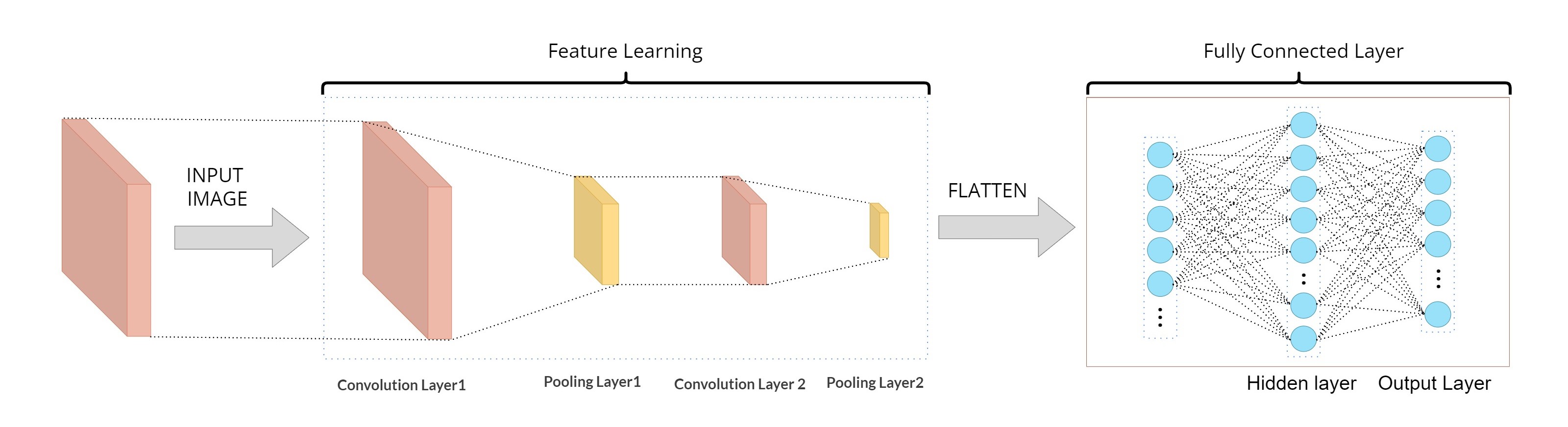
### 1. 建立卷積層與池化層
```python=
from keras.models import Sequential
from keras.layers import Dense,Dropout,Flatten,Conv2D,MaxPool2D
model = Sequential()
# Create CN layer 1
model.add(Conv2D(filters=16,
kernel_size=(5,5),
padding='same',
input_shape=(28,28,1),
activation='relu',
name='conv2d_1'))
# Create Max-Pool 1
model.add(MaxPool2D(pool_size=(2,2), name='max_pooling2d_1'))
# Create CN layer 2
model.add(Conv2D(filters=36,
kernel_size=(5,5),
padding='same',
input_shape=(28,28,1),
activation='relu',
name='conv2d_2'))
# Create Max-Pool 2
model.add(MaxPool2D(pool_size=(2,2), name='max_pooling2d_2'))
# Add Dropout layer
model.add(Dropout(0.25, name='dropout_1'))
```
### 2. 建立神經網路
* 建立平坦層
下面程式碼建立平坦層, 將之前步驟已經建立的池化層2, 共有 36 個 7x7 維度的影像轉換成 1 維向量, 長度是 36x7x7 = 1764, 也就是對應到 1764 個神經元:
```python=
model.add(Flatten(name='flatten_1'))
```
* 建立 Hidden layer
```python=
model.add(Dense(128, activation='relu', name='dense_1'))
model.add(Dropout(0.5, name='dropout_2'))
```
* 建立輸出層
最後建立輸出層, 共有 10 個神經元, 對應到 0~9 共 10 個數字. 並使用 softmax 激活函數 進行轉換 (softmax 函數可以將神經元的輸出轉換成每一個數字的機率):
```python=
model.add(Dense(10, activation='softmax', name='dense_2'))
```
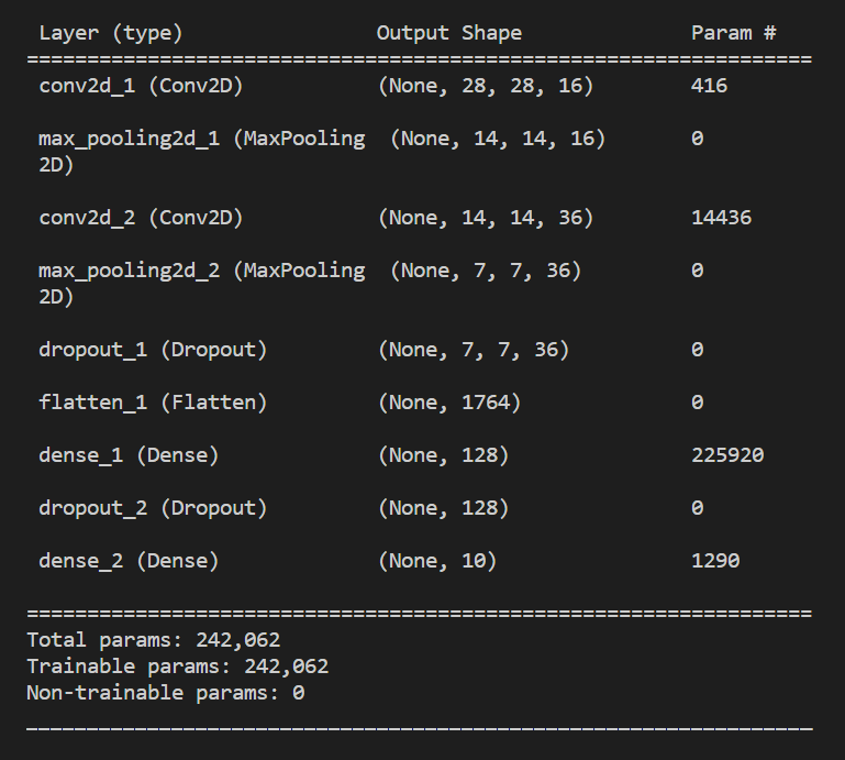
### 3. 查看模型
```python=
model.summary()
print("")
```
> 輸出:
> >>>
>
<BR>
<BR>
## 三、進行訓練
* 使用 Back Propagation 進行訓練。
### 1. 定義訓練並進行訓練
```python=
# 定義訓練方式
model.compile(loss='categorical_crossentropy', optimizer='adam', metrics=['accuracy'])
# 開始訓練
train_history = model.fit(x=X_Train4D_norm,
y=y_TrainOneHot, validation_split=0.2,
epochs=10, batch_size=300, verbose=1)
```
:::info
#### 在 compile 方法中:
* loss: 設定 Loss Function, 這邊選定 Cross Entropy 作為 Loss Function.
* optimizer: 設定訓練時的優化方法, 在深度學習使用 adam (Adam: A Method for Stochastic Optimization) 可以更快收斂, 並提高準確率.
* metrics: 設定評估模型的方式是 accuracy 準確率.
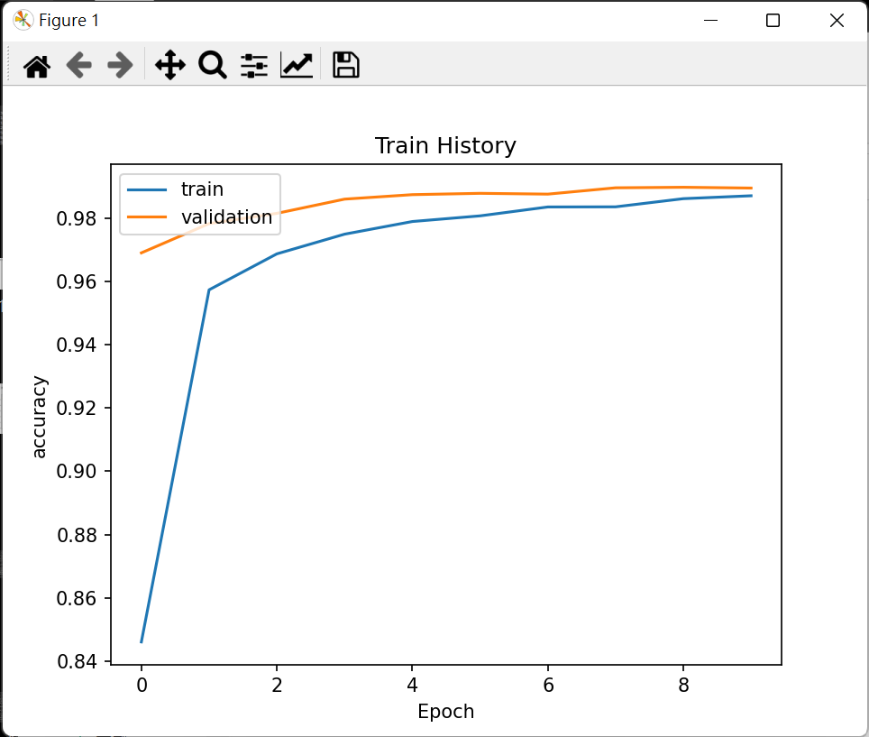
* STEP2. 畫出 accuracy 執行結果
* 之前的訓練步驟產生的 accuracy 與 loss 都會記錄在 train_history 變數.
:::
```python=
import matplotlib.pyplot as plt
def plot_image(image):
fig = plt.gcf()
fig.set_size_inches(2,2)
plt.imshow(image, cmap='binary')
plt.show()
def plot_images_labels_predict(images, labels, prediction, idx, num=10):
fig = plt.gcf()
fig.set_size_inches(12, 14)
if num > 25: num = 25
for i in range(0, num):
ax=plt.subplot(5,5, 1+i)
ax.imshow(images[idx], cmap='binary')
title = "l=" + str(labels[idx])
if len(prediction) > 0:
title = "l={},p={}".format(str(labels[idx]), str(prediction[idx]))
else:
title = "l={}".format(str(labels[idx]))
ax.set_title(title, fontsize=10)
ax.set_xticks([]); ax.set_yticks([])
idx+=1
plt.show()
def show_train_history(train_history, train, validation):
plt.plot(train_history.history[train])
plt.plot(train_history.history[validation])
plt.title('Train History')
plt.ylabel(train)
plt.xlabel('Epoch')
plt.legend(['train', 'validation'], loc='upper left')
plt.show()
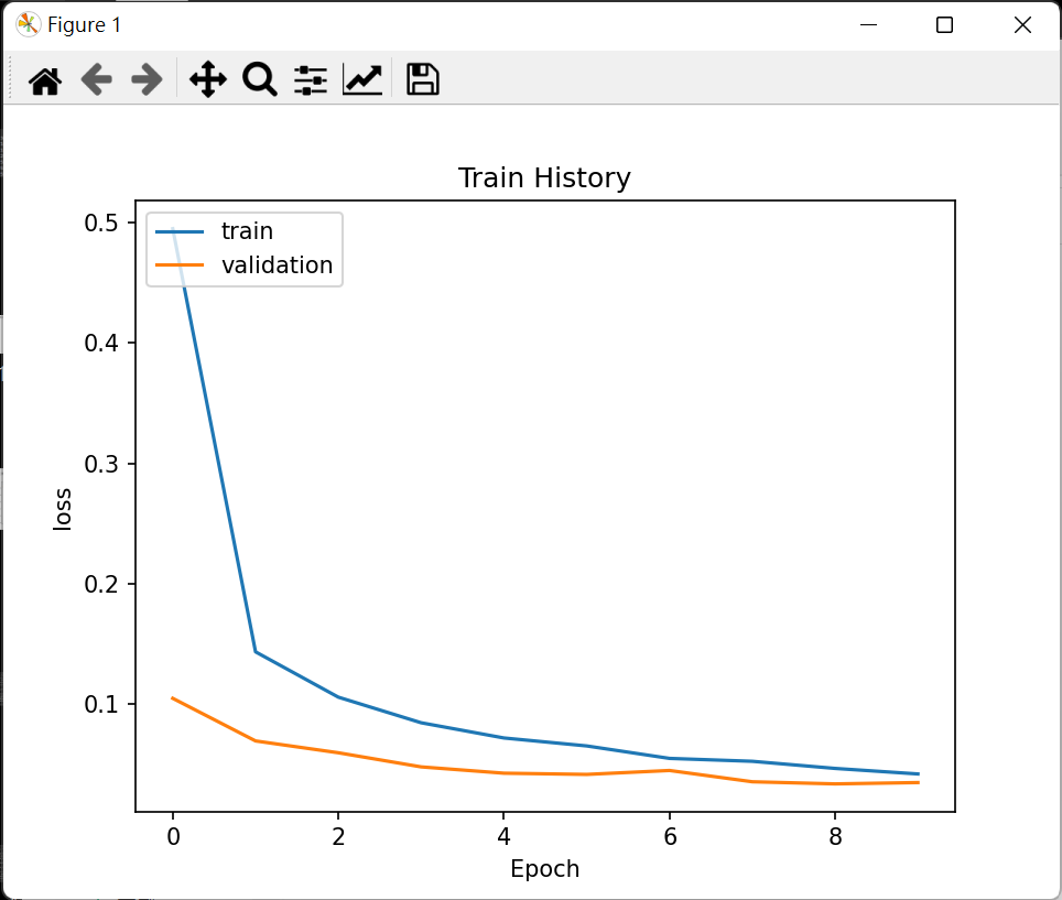
#使用函數 show_train_history 顯示 accuracy 在 train 與 evaluation 的差異與 loss 在 train 與 evaluation 的差異如下:
show_train_history(train_history,'accuracy','val_accuracy')
show_train_history(train_history, 'loss', 'val_loss')
```
> 輸出:
> >>>
>
<BR>
>>>
>
<BR>
<BR>
## 四、評估模型準確率與進行預測
#我們已經完成訓練, 接下來要使用 test 測試資料集來評估準確率。
### 1. 評估模型準確率
```python=
scores = model.evaluate(X_Test4D_norm, y_TestOneHot)
print()
print("\t[Info] Accuracy of testing data = {:2.1f}%".format(scores[1]*100.0))
```
> 輸出:
> >>> [Info] Accuracy of testing data = 99.1%
### 2. 預測結果
```python=
print("\t[Info] Making prediction of X_Test4D_norm")
prediction = model.predict(X_Test4D_norm)# Making prediction and save result to prediction
prediction = np.argmax(prediction,axis=1)
print()
print("\t[Info] Show 10 prediction result (From 240):")
print("%s\n" % (prediction[240:250]))
```
>輸出:
> >>> [Info] Making prediction of X_Test4D_norm
> >>> 313/313 [==============================] - 2s 6ms/step
> >>> [Info] Show 10 prediction result (From 240):
> >>> [5 9 8 7 2 3 0 4 4 2]
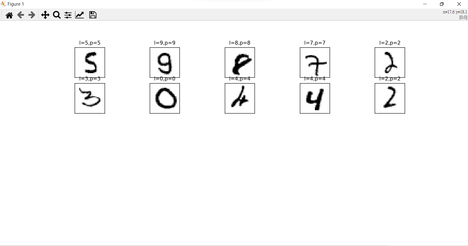
### 3. 顯示前 10 筆預測結果
```python=
plot_images_labels_predict(X_Test, y_Test, prediction, idx=240)
```
> 輸出:
> >>>
>
<BR>
<BR>
## 總結 (Conclusion)
了解網絡的結構與不同網絡層輸入輸出的張量的結構才能夠清楚地構建一個對的模型.
<BR>
---
# MNIST 手寫數字辨識資料集 RNN實作
## 一、導入函式庫
```python=
import numpy as np
from keras.datasets import mnist
from keras.utils import np_utils
from keras.models import Sequential
from keras.layers import SimpleRNN, Activation, Dense
from keras.optimizers import Adam
```
<br>
<br>
## 二、固定亂數種子,使每次執行產生的亂數都一樣
```python=
np.random.seed(1337)
```
<br>
<br>
## 三、載入 MNIST 資料庫的訓練資料,並自動分為『訓練組』及『測試組』
```python=
(X_train, y_train), (X_test, y_test) = mnist.load_data()
```
<br>
<br>
## 四、將 training 的 input 資料轉為3維,並 normalize 把顏色控制在 0 ~ 1 之間
```python=
X_train = X_train.reshape(-1, 28, 28) / 255.
X_test = X_test.reshape(-1, 28, 28) / 255.
y_train = np_utils.to_categorical(y_train, num_classes=10)
y_test = np_utils.to_categorical(y_test, num_classes=10)
```
<br>
<br>
## 五、建立簡單的線性執行的模型
```python=
model = Sequential()
```
<br>
<br>
## 六、加 RNN 隱藏層(hidden layer)
```python=
model.add(SimpleRNN(
# 如果後端使用tensorflow,batch_input_shape 的 batch_size 需設為 None.
# 否則執行 model.evaluate() 會有錯誤產生.
batch_input_shape=(None, 28, 28),
units= 50,
unroll=True,
))
```
<br>
<br>
## 七、加 output 層
```python=
model.add(Dense(units=10, kernel_initializer='normal', activation='softmax'))
```
<br>
<br>
## 八、編譯: 選擇損失函數、優化方法及成效衡量方式
```python=
model.compile(loss='categorical_crossentropy', optimizer='adam', metrics=['accuracy'])
#一批訓練多少張圖片
```python=
BATCH_SIZE = 50
BATCH_INDEX = 0
#訓練模型 4001 次
```python=
for step in range(1, 4001):
# data shape = (batch_num, steps, inputs/outputs)
X_batch = X_train[BATCH_INDEX: BATCH_INDEX+BATCH_SIZE, :, :]
Y_batch = y_train[BATCH_INDEX: BATCH_INDEX+BATCH_SIZE, :]
# 逐批訓練
loss = model.train_on_batch(X_batch, Y_batch)
BATCH_INDEX += BATCH_SIZE
BATCH_INDEX = 0 if BATCH_INDEX >= X_train.shape[0] else BATCH_INDEX
# 每 500 批,顯示測試的準確率
if step % 500 == 0:
# 模型評估
loss, accuracy = model.evaluate(X_test, y_test, batch_size=y_test.shape[0],
verbose=False)
print("test loss: {} test accuracy: {}".format(loss,accuracy))
```
> 輸出:
>>>> test loss: 0.7074328660964966 test accuracy: 0.762499988079071
>>> test loss: 0.4950987696647644 test accuracy: 0.8511000275611877
>>>> test loss: 0.4402388632297516 test accuracy: 0.8640999794006348
>>>> test loss: 0.37105119228363037 test accuracy: 0.8916000127792358
>>>> test loss: 0.31764569878578186 test accuracy: 0.90829998254776
>>> test loss: 0.3107646405696869 test accuracy: 0.9093000292778015
>>>> test loss: 0.2785736918449402 test accuracy: 0.9210000038146973
>>> test loss: 0.24084238708019257 test accuracy: 0.9318000078201294
<br>
<br>
## 九、預測(prediction)
```python=
X = X_test[0:10,:]
predictions = model.predict(X)
predictions = np.argmax(predictions,axis=1)
# get prediction result
print(predictions)
```
>輸出:
>>>>1/1 [==============================] - 0s 269ms/step
>>>>[7 2 1 0 4 1 4 9 6 9]
<br>
<br>
## 十、模型結構存檔
```python=
from keras.models import model_from_json
json_string = model.to_json()
with open("SimpleRNN.config", "w") as text_file:
text_file.write(json_string)
```
<br>
<br>
## 十一、模型訓練結果存檔
```python=
model.save_weights("SimpleRNN.weight")
scores = model.evaluate(X_test, y_test)
print()
print("\t[Info] Accuracy of testing data = {:2.1f}%".format(scores[1]*100.0))
```
> 輸出:
>>>>[Info] Accuracy of testing data = 93.4%
### RNN模型準確率為93.4%