# MNIST 手寫數字辨識資料集
## 一、下載 Mnist 資料
```python=
# 1.匯入 Keras 及相關模組
import numpy as np
import pandas as pd
from keras.utils import np_utils
# 用來後續將 label 標籤轉為 one-hot-encoding
np.random.seed(10)
# 2.下載 mnist data
from keras.datasets import mnist
# 3.讀取與查看 mnist data
(X_train_image, y_train_label), (X_test_image, y_test_label) = mnist.load_data()
print("\t[Info] train data={:7,}".format(len(X_train_image)))
print("\t[Info] test data={:7,}".format(len(X_test_image)))
```
>輸出:
>>>>[Info] train data= 60,000
>>>>[Info] test data= 10,000
<br>
<br>
## 二、查看訓練資料
```python=
# 1.訓練資料是由 images 與 labels 所組成
print("\t[Info] Shape of train data=%s" % (str(X_train_image.shape)))
print("\t[Info] Shape of train label=%s" % (str(y_train_label.shape)))
# 得:訓練資料是由 images 與 labels 所組成共有 60,000 筆, 每一筆代表某個數字的影像為 28x28 pixels.
# 2.建立 plot_image 函數顯示數字影像
import matplotlib.pyplot as plt
def plot_image(image):
fig = plt.gcf()
fig.set_size_inches(2,2)
plt.imshow(image, cmap='binary') # cmap='binary' 參數設定以黑白灰階顯示.
plt.show()
# 3.執行 plot_image 函數查看第 0 筆數字影像與 label 資料
plot_image(X_train_image[0])
print(y_train_label[0])
# 得:呼叫 plot_image 函數, 傳入 X_train_image[0], 也就是順練資料集的第 0 筆資料, 顯示結果可以看到這是一個數字 5 的圖形
```
> 輸出:
>>>>[Info] Shape of train data=(60000, 28, 28)
>>>>[Info] Shape of train label=(60000,)
<br>
>>>>
>
<br>
>>>>5
<br>
<br>
## 三、查看多筆訓練資料 images 與 labels
```python=
# 1.建立 plot_images_labels_predict() 函數
# 為了後續能很方便查看數字圖形, 真實的數字與預測結果
def plot_images_labels_predict(images, labels, prediction, idx, num=10):
fig = plt.gcf()
fig.set_size_inches(12, 14)
if num > 25: num = 25
for i in range(0, num):
ax=plt.subplot(5,5, 1+i)
ax.imshow(images[idx], cmap='binary')
title = "l=" + str(labels[idx])
if len(prediction) > 0:
title = "l={},p={}".format(str(labels[idx]), str(prediction[idx]))
else:
title = "l={}".format(str(labels[idx]))
ax.set_title(title, fontsize=10)
ax.set_xticks([]); ax.set_yticks([])
idx+=1
plt.show()
plot_images_labels_predict(X_train_image, y_train_label, [], 0, 10)
```
> 輸出:
>>>>
<br>
<br>
## 四、多層感知器模型資料前處理
* 建立 多層感知器模型 (MLP), 須先將 images 與 labels 的內容進行前處理, 才能餵進去 Keras 預期的資料結構.
```python=
# 1.features (數字影像的特徵值) 資料前處理
# 先將 image 以 reshape 轉換為二維 ndarray 並進行 normalization (Feature scaling):
x_Train = X_train_image.reshape(60000, 28*28).astype('float32')
x_Test = X_test_image.reshape(10000, 28*28).astype('float32')
print("\t[Info] xTrain: %s" % (str(x_Train.shape)))
print("\t[Info] xTest: %s" % (str(x_Test.shape)))
# Normalization
x_Train_norm = x_Train/255
x_Test_norm = x_Test/255
```
> 輸出:
>>>>[Info] xTrain: (60000, 784)
>>>>[Info] xTest: (10000, 784)
<br>
```python=
# 2.labels (影像數字真實的值) 資料前處理
y_TrainOneHot = np_utils.to_categorical(y_train_label)
# 將 training 的 label 進行 one-hot encoding
y_TestOneHot = np_utils.to_categorical(y_test_label)
# 將測試的 labels 進行 one-hot encoding
# 檢視 training labels 第一個 label 的值
print (y_train_label[0])
# 檢視第一個 label 在 one-hot encoding 後的結果, 會在第六個位置上為 1, 其他位置上為 0
print(y_TrainOneHot[:1])
```
> 輸出:
>>>>5
>>>>[[0. 0. 0. 0. 0. 1. 0. 0. 0. 0.]]
:::info
label 標籤欄位原本是 0-9 數字, 而為了配合 Keras 的資料格式, 必須進行 One-hot-encoding 將之轉換為 10 個 0 或 1 的組合, 例如數字 7 經過 One-hot encoding 轉換後是 0000001000, 正好對應到輸出層的 10 個神經元.
:::
<br>
<br>
## 五、建立模型
* 建立多層感知器 Multilayer Perceptron 模型:
輸入層 (x) 共有 28x28=784 個神經元, Hidden layers (h) 共有 256 層; 輸出層 (y) 共有 10 個 神經元
```python=
from keras.models import Sequential
from keras.layers import Dense
model = Sequential() # Build Linear Model
model.add(Dense(units=256, input_dim=784, kernel_initializer='normal', activation='relu')) # Add Input/hidden layer
model.add(Dense(units=10, kernel_initializer='normal', activation='softmax')) # Add Hidden/output layer
print("\t[Info] Model summary:")
model.summary()
print("")
```
> 輸出:
>>>>
<br>
<br>
## 六、進行訓練
* 建立深度學習模型後, 使用 Backpropagation 進行訓練
```python=
# 1.定義訓練方式
# 在訓練模型之前, 我們必須先使用 compile 方法, 對訓練模型進行設定
model.compile(loss='categorical_crossentropy', optimizer='adam', metrics=['accuracy'])
```
:::info
* loss: 設定 loss function, 在深度學習通常使用 cross_entropy (Cross entropy) 交叉摘順練效果較好.
* optimizer: 設定訓練時的優化方法, 在深度學習使用 adam 可以讓訓練更快收斂, 並提高準確率.
* metrics: 設定評估模型的方式是 accuracy (準確率)
:::
```python=
# 2.開始訓練
train_history = model.fit(x=x_Train_norm, y=y_TrainOneHot, validation_split=0.2, epochs=10, batch_size=200, verbose=2)
```
:::info
#### 上面訓練過程會儲存於 train_history 變數中:
* x=x_Train_norm: features 數字的影像特徵值 (60,000 x 784 的陣列).
* y=y_Train_OneHot: label 數字的 One-hot encoding 陣列 (60,000 x 10 的陣列)
* validation_split = 0.2: 設定訓練資料與 cross validation 的資料比率. 也就是說會有 0.8 * 60,000 = 48,000 作為訓練資料; 0.2 * 60,000 = 12,000 作為驗證資料.
* epochs = 10: 執行 10 次的訓練週期.
* batch_size = 200: 每一批次的訓練筆數為 200
* verbose = 2: 顯示訓練過程. 共執行 10 次 epoch (訓練週期), 每批 200 筆, 也就是每次會有 240 round (48,000 / 200 = 240). 每一次的 epoch 會計算 accuracy 並記錄在 train_history 中.
:::
```python=
# 3.建立 show_train_history 顯示訓練過程
# 訓練步驟會將每一個訓練週期的 accuracy 與 loss 記錄在 train_history 變數
# 讀取 train_history 以圖表顯示訓練過程:
import matplotlib.pyplot as plt
def show_train_history(train_history,train,validation):
plt.plot(train_history.history[train])
plt.plot(train_history.history[validation])
plt.title('Train history')
plt.ylabel('train')
plt.xlabel('epoch')
# 設置圖例在左上角
plt.legend(['train','validation'],loc='upper left')
plt.show()
show_train_history(train_history,'accuracy','val_accuracy')
show_train_history(train_history,'loss','val_loss')
```
> 輸出:
>>>>
<br>
>>>>
:::info
如果 "accuracy 訓練的準確率" 一直提升,但是 "val_accuracy 的準確率" 卻一直沒有增加,可能是 Overfitting 的現象.
在完成所有 (epoch) 訓練週期後,在後面還會使用測試資料來評估模型準確率, 這是另外一組獨立的資料,所以計算準確率會更客觀.
#### 總共執行 10 個 Epoch 訓練週期, 發現:
* 不論訓練與驗證, 誤差越來越低.
* 在 Epoch 訓練後期, "loss 訓練的誤差" 比 "val_loss 驗證的誤差" 小.
:::
<br>
<br>
## 七、以測試資料評估模型準確率與預測
* 已經完成訓練模型, 現在要使用 test 測試資料來評估模型準確率.
```python=
# 1.評估模型準確率
# 使用下面代碼評估模型準確率:
scores = model.evaluate(x_Test_norm, y_TestOneHot)
print()
print("\t[Info] Accuracy of testing data = {:2.1f}%".format(scores[1]*100.0))
```
>>>>[Info] Accuracy of testing data = 97.6%
```python=
# 2.進行預測
print("\t[Info] Making prediction to x_Test_norm")
prediction = model.predict(x_Test_norm)
prediction = np.argmax(prediction,axis=1)
print()
print("\t[Info] Show 10 prediction result (From 240):")
print("%s\n" % (prediction[240:250]))
plot_images_labels_predict(X_test_image, y_test_label, prediction, idx=240)
```
>>>>[Info] Making prediction to x_Test_norm
>>>313/313 [==============================] - 0s 1ms/step
>>>[Info] Show 10 prediction result (From 240):
> [5 9 8 7 2 3 0 6 4 2]
:::info
prediction = model.predict_classes(x_Test_norm)
predict_classes()函數在 TensorFlow 2.6 版本中被移除了以:
1. prediction = (model.predict(x_Test_norm) > 0.5).astype("int32")
2. prediction = model.predict(x_Test_norm)
prediction = np.argmax(prediction,axis=1)
最後選擇第二選擇,因為前者為二進制
:::
<br>
<br>
## 八、顯示混淆矩陣 (Confusion matrix)
* 如果想要進一步知道建立的模型中,那些數字預測準確率最高,那些數字最容易混淆,此時可以使用混淆矩陣(Confusion matrix).
* 在機器學習領域,特別是統計分類的問題,混淆矩陣(也稱為 error matrix)是一種特定的表格顯示方式,可以以視覺化的方式,了解Supervisored Learning的結果,看出訓練出來的模型在各個類別的表現狀況.
```python=
# 1.使用 pandas crosstab 建立混淆矩陣 (Confusion matrix)
print("\t[Info] Display Confusion Matrix:")
import pandas as pd
print("%s\n" % pd.crosstab(y_test_label, prediction, rownames=['label'], colnames=['predict']))
```
>輸出:
>>>>
:::info
* 對角線是預測結果正確的數字, 我們發現類別 "1" 的預測準確率最高共有 1,125 筆; 類別 "5" 的準確率最低共有 852 筆.
* 其他非對角線的數字, 代表將某一類別預測成其他類別的錯誤. 例如將類別 "5" 預測成 "3" 共發生 12 次.
:::
```python=
# 2.建立真實與預測的 dataframe
# 如找出那些 label 結果為 "5" 的結果被預測成 "3" 的資料, 所以建立的下面的 dataframe:
df = pd.DataFrame({'label':y_test_label, 'predict':prediction})
df[:2] # 顯示前兩筆資料
```
```python=
# 3.查詢 label=5; prediction=3 的資料
# Pandas Dataframe 可以讓你很方便的查詢資料:
out = df[(df.label==5) & (df.predict==3)] # 查詢 label=5; predict=3 的 records
out.__class__ # 輸出是另一個 DataFrame
print(out)
```
>輸出:
>>>>
>
```python=
# 4.查看第 340 筆資料
plot_images_labels_predict(X_test_image, y_test_label, prediction, idx=340, num=1)
```
>輸出:
>>>>
>
### 到目前為止模型準確率為97.8%
<br>
<br>
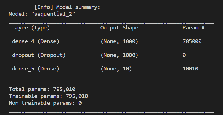
## 九、隱藏層增加為 1000 個神經元
* 為了增加準確率, 我們將 Hidden layers 的數目從 256 提升到 1000 個神經元:
```python=
#1. 修改模型
from keras.models import Sequential
from keras.layers import Dense
model = Sequential() # Build Linear Model
model.add(Dense(units=1000, input_dim=784, kernel_initializer='normal', activation='relu')) # Modify hidden layer from 256 -> 1000
model.add(Dense(units=10, kernel_initializer='normal', activation='softmax'))
print("\t[Info] Model summary:")
model.summary()
print("")
show_train_history(train_history,'accuracy','val_accuracy')
```
>輸出:
>>>>
>
<br>
>>>
>
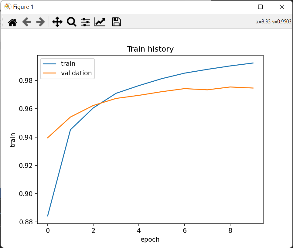
:::info
#### 檢視執行結果
從下面的 "accuracy" vs "validation accuracy" 的圖可以看出兩者差距拉大 (training accuracy > validation accuracy), 說明 Overfitting 問題變嚴重
:::
<br>
<br>
## 十、多層感知器加入 DropOut 功能以避免 Overfitting
* 為了解決 Overfitting 問題, 接下來會加入 Dropout 功能, 以避免 Overfitting
Dropout 是指在模型訓練時隨機讓網絡某些隱含層節點的權重不工作,不工作的那些節點可以暫時認為不是網絡結構的一部分,但是它的權重得保留下來(只是暫時不更新而已),因為下次樣本輸入時它可能又得工作了。
```python=
#1. 修改隱藏層加入 DropOut 功能
from keras.models import Sequential
from keras.layers import Dense
from keras.layers import Dropout # ***** Import DropOut mooule *****
model = Sequential()
model.add(Dense(units=1000, input_dim=784, kernel_initializer='normal', activation='relu'))
model.add(Dropout(0.5)) # ***** Add DropOut functionality *****
model.add(Dense(units=10, kernel_initializer='normal', activation='softmax'))
print("\t[Info] Model summary:")
model.summary()
print("")
show_train_history(train_history,'accuracy','val_accuracy')
```
>輸出:
>>>>
>
<br>
>>>
>
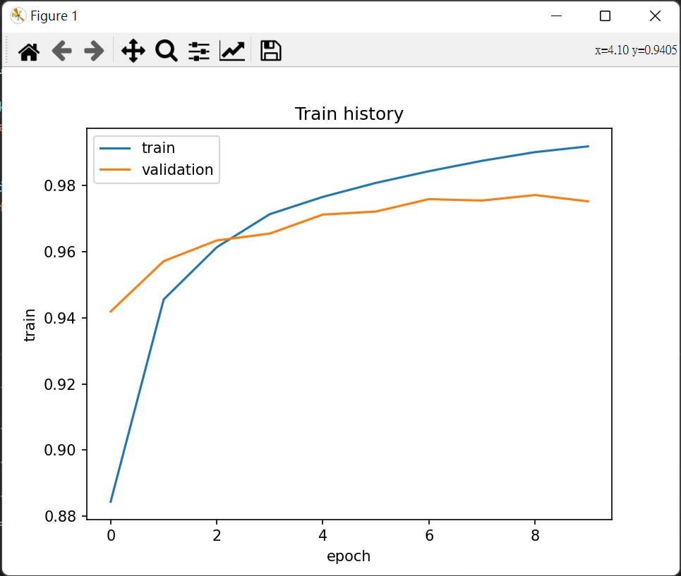
:::info
#### 檢視進行訓練後結果
最後一個 Epoch 的執行結果可以發現 acc 與 val_acc 接近許多, 說明 Overfitting 問題有被解決.
:::
<br>
<br>
## 十一、建立多層感知器模型 (包含兩個 Hidden Layers)
* 為了進一步提升準確率, 可提升多元感知器 Hidden layer 的層數.
```python=
#1. 變更模型使用兩個 Hidden Layers 並加入 DropOut 功能
from keras.models import Sequential
from keras.layers import Dense
from keras.layers import Dropout # Import DropOut mooule
model = Sequential() # Build Linear Model
model.add(Dense(units=1000, input_dim=784, kernel_initializer='normal', activation='relu')) # Add Input/ first hidden layer
model.add(Dropout(0.5)) # Add DropOut functionality
model.add(Dense(units=1000, kernel_initializer='normal', activation='relu')) # Add second hidden layer
model.add(Dropout(0.5)) # Add DropOut functionality
model.add(Dense(units=10, kernel_initializer='normal', activation='softmax')) # Add Hidden/output layer
print("\t[Info] Model summary:")
model.summary()
print("")
show_train_history(train_history,'accuracy','val_accuracy')
```
>輸出:
>>>>
>
<br>
>>>
>
:::info
#### 進行訓練並察看結果
由 accuracy 圖可以看出 training accuracy 與 validation accuracy 已經相當接近, 說明 Overfitting 的影響又被改善了
:::
### CNN模型準確率為97.8%
## 結論
多層感知器 Multilayer perceptron 模型,辨識手寫字嘗試將模型加寬加深,加入drop以提高準確度,避免 overfitting ,但多層感知器有其極限,若要提高準確度,就要使用卷積神經網路 CNN .
<br>
<br>