---
# System prepended metadata
title: '形式化证明浅析: 第一个程序证明'
---
## 概述
在计算机领域中,形式证明是时常被讨论的话题。伴随着 LLM 时代的到来,很多工程师和计算机科学家都认为形式化证明将逐渐成为未来软件标配,工程师可能只需要编写软件的 spec 然后 LLM 会编写代码然后利用形式化证明方法验证编写代码的正确性。
经典的分布式系统书籍 DDIA 的作者在 2025 年 12 月编写了博客 [Prediction: AI will make formal verification go mainstream](https://martin.kleppmann.com/2025/12/08/ai-formal-verification.html),认为 LLM 辅助下形式化证明将成为主流。z3 SMT 求解器的作者之一 [Leonardo de Moura](https://leodemoura.github.io/) 在最近的博客 [When AI Writes the World’s Software, Who Verifies It?](https://leodemoura.github.io/blog/2026/02/28/when-ai-writes-the-worlds-software.html) 也说明了形式化证明的重要性,并指明了未来可以通过使用 Lean 4 语言通向基于 LLM 的自动化形式化证明。
另外,对形式化证明感到兴奋的是数学家,陶哲轩始终是形式化证明的支持者。陶哲轩的经典著作 Analysis I 使用了 Lean 4 进行形式化证明,具体可以参考 [A Lean companion to “Analysis I”](https://terrytao.wordpress.com/2025/05/31/a-lean-companion-to-analysis-i/),而且陶哲轩目前的 [Youtube 频道](https://www.youtube.com/@TerenceTao27) 内的所有视频目前都是关于 Lean 4 的。
对于形式化证明的未来最好的想象来自 Stephen Diehl 的博客 [The Future of Maths May Be Deeply Weird](https://www.stephendiehl.com/posts/future_math_weird/)。该文章内有一段如下:
> Stretching our imagination further, we can envision a far future where this technology reaches its zenith. A dedicated data center could be tasked with a grand challenge, like the Riemann hypothesis. After weeks of processing, it might return a positive result: a complete, machine-checkable proof. Yet, the proof's internal structure could be so byzantine, so alien in its logic, that no human could ever hope to grasp its intuitive thrust, much like the computer-assisted proof of the Four Color Theorem or the controversy surrounding the Mochizuki proof of the ABC conjecture. This would usher in a disquieting new reality, a world where machines, not unlike the [hyper-intelligent Minds](https://www.youtube.com/watch?v=g2T-TStvRNM) from Iain M. Banks' Culture series, venture into intellectual territories forever beyond human comprehension. We would "know" (epistomigical concerns aside) and accept certain mathematical truths, but as humans we would never intuit or understand why they are true. And that is a very different world in which science happens.
但是本文并不是一篇 Lean 4 教程,本文也不会涉及数学定理方面的形式化证明,本文仍将专注在计算机程序的形式化证明方面,而且我们会使用非常朴素的方法,我们会将一段程序的正确性转化为一个逻辑命题的正确性问题,并且我们不会使用手动方法证明该逻辑命题的正确性,这些命题实际上也可以容易被手动证明,但是手动证明这些命题需要一些额外的逻辑学知识,为了降低本文的阅读难度,我们将使用求解器简化。本文使用的是 [z3 prover](https://github.com/Z3Prover/z3)。
从先进性角度来看,使用 z3 或其他 solver 进行半自动式的形式化证明似乎不是充分先进的,目前的学界共识是使用 Lean 4 才是未来。但本文核心是介绍代码形式化证明的数学原理,这些原理实际上可以直接迁移到 Lean 4 内部,并且本文只会在形式化证明的最后一步求解逻辑命题时使用 z3,即使读者对 z3 等 SMT 求解器抱有鄙视态度,仍可以在本文的大量的手动证明部分获得一些知识。
> 为什么对基于 `z3` 的形式化证明目前并不被推崇?`z3` 以及 Lean 4 的开发者 Leonardo de Moura 在最近的博客 [Who Watches the Provers?](https://leodemoura.github.io/blog/2026-3-16-who-watches-the-provers/) 内给出了答案。简单来说,使用 z3 等 SMT 求解器实现是可能存在问题的,所以验证结果并不一定可靠
另外,笔者所有的知识实际上都来自著名形式化证明教科书 [The Calculus of Computation by Aaron Bradley and Zohar Manna](https://theory.stanford.edu/~arbrad/book.html),假如读者对本文内任何只给出名称但没有展开解释的概念感兴趣,你可以直接在书中搜索该名词。本文内使用 **参考书** 一词代指该书。该书的电子版本不难在一些网站内找到,更加建议读者购买纸质版本。
## 初探 SMT
对于 `z3` 的安装,最常见是利用 Python 的 `z3-solver` 安装,该包内包含 `z3` 二进制编译结果以及使用 Python 调用 z3 的 API。或者读者也可以直接使用 `brew` 等包管理器安装 `z3`,具体可以自行搜索包管理器的仓库。还有一种更加简单的方法,即直接使用在线版本的 z3,比如 [FM Playground](https://play.formal-methods.net/),本文中的所有逻辑命题都可以在在线平台内求解获得结果。为了方便,本文将使用 SMT Solver 领域的一等公民类 Common Lisp 的 [smt2](https://smt-lib.org/),这是 SMT Solver 领域的标准规范语言,很多求解器都支持该语言表示的问题描述,比如 [z3](https://github.com/Z3Prover/z3) 和 [yices2](https://github.com/SRI-CSL/yices2),所以假如读者有自己喜欢的求解器,也可以直接使用,而不一定使用本文中提到的 z3 求解器。
在介绍后续内容前,我们可以补充一些 Propositional Logic 内的基础概念,此处我们主要介绍任何命题都可以是 *satisfiable* 或者 *valid* 的。所谓 *satisfiable* 是指存在某种条件使得命题成立;而 *valid* 则更加严格,要求命题必须在所有条件下都是恒成立的。在具体问题上,假如我们希望“求解”某一个命题,那么可以使用 *satisfiable* 属性,实际上 `z3` 只支持使用 `(check-sat)` 检查命题的 satisfiable 属性,该函数的输出为 `sat` 和 `unsat`。
但值得注意的是,satisfiable 和 valid 实际上是双向概念,我们可以使用反证方法简单的将验证 valid 转化为验证 satisfiable,即 $F$ 是 valid 的当且仅当 $\neg F$ 是 unsatisfiable。
比如我们可以验证如下命题是 satisfiable 并且也是 valid 的:
$$
F: A \to B \to C \iff (A \land B) \to C
$$
上述命题中的 $\iff$ 表示当且仅当(iff),我们简单认为就是 `=` 含义。我们先判断该命题是否存在一种赋值使得 F 为 true。此处我们使用更加底层的 smt2 语言进行编写:
```lisp
(declare-const A Bool)
(declare-const B Bool)
(declare-const C Bool)
(define-fun f () Bool
(=
(=> A (=> B C))
(=> (and A B) C)))
(assert f)
(check-sat)
(get-model)
```
上述 `(assert f)` 的语义是将 `f` 放入最后的待求解命题中,有时候,我们会遇到多个 `assert` 的情况,比如这种情况:
```lisp
(assert F1)
(assert F2)
(assert F3)
```
此时求解器会认为目前的待求解命题是 $F1 \land F2 \land F3$,`assert` 声明的约束会被最终合取构成一个 CNF([Conjunctive normal form](https://en.wikipedia.org/wiki/Conjunctive_normal_form))。CNF 具有很多良好的性质,求解器主流的求解算法只能执行在 CNF 类型的表达式上,比如大名鼎鼎的 [DPLL 算法](https://en.wikipedia.org/wiki/DPLL_algorithm) 以及 [DPLL(T) 算法](https://en.wikipedia.org/wiki/DPLL(T)),这些算法其实就是求解器自动验证逻辑命题时的核心算法。这些内容我们会在未来介绍求解器底层时进行涉及。
`(check-sat)` 就是检查 `assert` 语句构建的逻辑命题是否 satisfiable,其输出结果为 `sat` 和 `unsat`。而 `(get-model)` 会在 `sat` 情况下给出命题内变量的赋值(更加专业的名词是 *interpretation*)。上述 smt2 在求解器内获得的结果如下:
```lisp
sat
(
(define-fun A () Bool
false)
(define-fun B () Bool
false)
(define-fun C () Bool
false)
(define-fun f () Bool
(= (=> A (=> B C)) (=> (and A B) C)))
)
```
`sat` 是 `(check-sat)` 的输出,而后续的内容是 `(get-model)` 的输出。我们可以看到当 A = false, B = false, C = false 时,命题 $F$ 成立。在 Propositional Logic 领域,我们一般会使用如下符号表示命题内的变量赋值:
$$
I: \{A \mapsto \mathrm{false}, B \mapsto \mathrm{false}, C \mapsto \mathrm{false}\}
$$
假如使用当前 $I$ 可以使得命题 $F$ 为 true,我们会使用 $I \models F$ 表示。实际上,命题 F 也是 valid 的,正如上文所述,我们只需要检查 $I \models \neg F$ 的 satisfiable 情况,我们只需要将之前代码中的 `(assert f)` 修改为 `(assert (not f))` 即可,获得的结果为 `unsat`,这说明实际上命题 $F$ 在任何 interpretation 下都是恒成立的。
读者可以自行证明另一个经典结论:
$$
F: A \to B \iff \neg (A \land \neg B)
$$
手动证明可以直接列出上述命题的真值表。当然,直接使用 smt2 翻译上述命题丢给求解器求解。另外补充一下,在手动证明 $F$ 的 valid 属性时,我们会首先假设 $I \not\models F$,然后使用一种被称为 Semantic Arguments 的技术。这种技术存在一套规则集,我们可以调用规则集反复处理命题,直到发现处理获得的结果内存在矛盾(contradiction) 为止。我们会在未来介绍底层知识时补充该内容,假如读者面前感兴趣,请阅读参考书的 **1.3.2 Semantic Arguments** 一节。
接下来,我们在逻辑命题内引入 $\forall$ 和 $\exists$ 将简单的 Propositional Logic 拓展为 First-Order Logic(FOL)。其中 $\forall$ 与 $\exists$ 的定义如下:
1. 存在量词 $\exists x. F[x]$ 表示存在一个 $x$ 使得 $F[x]$
2. 全称量词 $\forall x. F[x]$ 表示对于所有的 $x$,$F[x]$
除了引入上述量词外,FOL 也包含了额外的几项(terms):
1. constant 常量
2. variable 变量,默认情况下变量可以任意取值,但也可以受量词约束
3. function 函数,如 $f(a)$ 或者更加复杂的 $f(g(x, f(b)))$ 等
举一个简单的例子:
$$
(\forall x. p(x)) \iff (\neg \exists x. \neg p(x))
$$
此处的 $p$ 是一个函数,我们甚至不知道 $p$ 的具体实现,但我们仍可以证明上述命题是 valid 的。这种不知道实现的函数一般被称为 uninterpreted functions,缩写为 `UF`。上述命题可以被翻译为:
```lisp
(set-logic UF)
(declare-sort A 0)
(declare-fun p (A) Bool)
(assert
(not
(= (forall ((x A)) (p x))
(not (exists ((x A)) (not (p x)))))))
(check-sat)
```
此处我们使用了额外的 `(set-logic UF)`,实际上该命令也可以不使用。z3 等求解器支持多种求解模式,此处的 `UF` 允许求解器求解带有未解释函数的逻辑命题,实际上所谓的求解模式与下文即将介绍的 theories 是有关的。另一个就是 `(declare-sort A 0)`。此处我们定义了一个 `sort` 类型,这类似编程中的泛型,实际上 `Int` / `Bool` 等 smt2 内建类型也属于 sort 类型。此处的 `(declare-sort A 0)` 中的 `0` 代表当前 sort 初始化时接受的参数数量(arity)。我们声明类型 `A` 的目的是为了使得 `x` 是充分抽象的,这样可以使得上述命题充分广泛。
> `sort` 的名称来自逻辑学的 Many-sorted logic 分支,笔者对该领域也并不熟悉,读者如果对此分支感兴趣可以阅读 [此 PPT](http://tsinghualogic.net/events/2014/easllc/wp-content/uploads/2014/03/China_MSL_20142.pdf)
实际上即使包含如此多的未解释函数以及一个不完全确定类型的 `x`,SMT 求解器仍可以进行求解,上述 smt2 语言的输出结果为 `unsat`,说明命题 $(\forall x. p(x)) \iff (\neg \exists x. \neg p(x))$ 是 valid 的。
有了上述知识后,我们就可以真正了解 SMT 的内容。SMT 的全程是 Satisfiability modulo theories。我们在上文介绍了 *Satisfiability* 一词的含义,而 *modulo* 实际上是一个介词,此处并不是计算机科学中的模除计算,在早期的 SMT 讨论中,我们可以看到如下语句
> According to one dictionary, “modulo” means “correcting or adjusting for something.” This is an appropriate definition for its use in satisfiability modulo theories:
>
> First-order logic defines a notion of satisfiability for arbitrary formulas. In SMT, we use the same definition of satisfiability, but *adjusted* by restricting the set of models we consider to those that also satisfy the theories involved.
>
> 转引自 [SAT/SMT by Example](https://smt.st/)
所以 SMT 的含义其实使用使用 Theories 修正的 Satisfiability 问题。那么 Theories 是什么?我们一般会使用 First-Order Theories。对于任何 theory T,其都是由以下两部分构成:
1. signature $\Sigma$ 是一组常数、函数或者 predicate symbols(可以认为是一种输出布尔值的特殊函数)
2. axioms $\mathcal{A}$ 代表一组定理,我们可以在验证逻辑命题的过程中使用该组定理
一个较为知名的 thoery 是 theory of Peano arithmetic(实际上就是大名鼎鼎的皮亚诺公理体系),数学符号为 $T_{\mathrm{PA}}$。
$$
\Sigma_{\mathrm{PA}}: \{0, 1, +, \cdot, =\}
$$
其中 $0, 1$ 都是常数,而加法($+$) 和乘法($\cdot$) 都是 binary function,而 $=$ 是 binary predicate。下图展示了所有的 axioms:
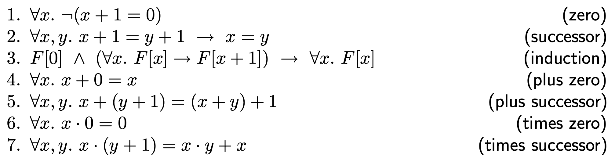
实际上皮亚诺公理系统严谨描述了自然数,在陶哲轩编写的实分析教程中,皮亚诺公理系统是第一节的内容。大部分 theory 下命题的 decidable 属性都是经过研究的。这里遇到了 decidable 属性,该属性对于学习过计算复杂性理论的读者可能并不陌生,这里给出一个不严谨的定义,所谓的 decidable 是指存在算法可以判断命题是否正确,对于 decidable 更深入的了解,读者可以通过阅读参考书目的 **2.6.2 Decidability** 或者简单阅读 complexityzoo 的 [Petting Zoo](https://complexityzoo.net/Petting_Zoo#Computing_and_Deciding_Problems) 条目。
> 大部分涉及可判定性的概念描述中都会使用 formal language 等前置概念,读者可以在自动机理论(Automata) 的书籍(比如《自动机理论、语言和计算导论》,其英文名为 *Introduction to Automata Theory, Languages, and Computation*,该书作者获得了图灵奖) 内找到更多有趣的介绍。假如读者不想从自动机理论角度进行严肃学习,那么也可以选择阅读《集异璧》,该书在第一章就介绍了“判定过程”
不幸的是,$T_{\mathrm{PA}}$ 的 Satisfiability 和 validity都是 undecidable,这与哥德尔第一不完备定理有关。但是存在一些更加严格的 thory 是可以判定的,比如我们在计算机领域中最常使用的 theory of Presburger arithmetic $T_{\mathbb{N}}$
$$
\Sigma_{\mathbb{N}}: \{0, 1, +, =\}
$$
注意此处没有乘法,对于整数乘法,熟悉数论的读者一定会想到丢番图方程以及希尔伯特第十问题,在皮亚诺算法系统内构建一个丢番图方程使得没有任何办法判定该方程是否有解,所以 $T_{\mathbb{N}}$ 直接不允许进行乘法计算(此处的乘法计算实际上指不允许进行 $x \cdot x$ 或者 $x \cdot y$ 的计算,此处的 $x$ 和 $y$ 都是变量,我们仍可以进行 $2x$ 这种计算,因为 $2x = x + x$)。与 $T_{\mathrm{PA}}$ 的公理系统类似,但是 $T_{\mathbb{N}}$ 的公理系统不包含 `times zero` 和 `times successor` 两条涉及乘法的公理。
> 在《永恒的图灵》一书中,第一章节就是希尔伯特第十问题的介绍,该章节的作者为希尔伯特第十问题的解决提供了重要的理论基础
在 1929 年,Presburger 就已经证明了 $T_{\mathbb{N}}$ 是可判定的。与 $T_{\mathbb{N}}$ 密切相关的且在计算机领域中最常被使用的是 theory of integers ${T_{\mathbb{Z}}}$:
$$
\Sigma_{\mathbb{Z}}: \{\dots, -2, -1, 0, 1, 2, \dots, -3 \cdot, -2 \cdot, 2 \cdot, 3 \cdot, +, -, = ,>\}
$$
此处额外引入了 $-2$ 等负整数,$3 \cdot$ 表示的乘法,所以在 $T_{\mathbb{Z}}$ 内,我们可以直接写 $2 \cdot x$ 类似的内容,还额外引入了 $=$ 和 $>$ 作为 binary predicates function。实际上,$T_{\mathbb{Z}}$ 和 $T_{\mathbb{N}}$ 之间的命题可以互相转换,所以 $T_{\mathbb{Z}}$ 也是可判定的。更加具体说存在一种被称为 Cooper's Algorithm 可以判定 $T_{\mathbb{Z}}$ 的 validity,但是计算机复杂度较高,我们会在本节末尾给出汇总。
> 补充材料: 读者可以阅读 Z3 Theory 下的 [Arithmetic](https://microsoft.github.io/z3guide/docs/theories/Arithmetic) 一节了解更多 z3 求解器内部对于 $T_{\mathbb{Z}}$ 以及相关数学系统的处理
一些与计算机领域更加密切相关的就是一些数据结构的 theory。比较著名的是 RDS(recursive data structures) 和 Array。在 RDS 中,最有名的是 $T_{\mathrm{cons}}$,这是一种在函数式编程语言中常见的表示列表的数据类型。在 Elixir 和 Haskell 内的 `list` 都与本文介绍的 $T_{\mathrm{cons}}$ 有关。$T_{\mathrm{cons}}$ 的 signature 如下:
$$
\Sigma_{\mathrm{cons}}: \{\text{cons}, \text{car}, \text{cdr}, \text{atom}, =\}
$$
其中 `cons` 是一个 binary function,比如 `cons(a, b)` 代表 `a` 和 `b` 可以拼接为一个列表。以下 Elixir 代码内的 `|` 可以视为 `cons` 函数,我们可以看到反复调用 `cons` 就可以构建一个列表:
```elixir
iex> [1 | [2 | [3 | []]]]
[1, 2, 3]
```
而 `car` 和 `cdr` 都是 unary function,含义为 `car(cons(a, b)) = a` 而 `cdr(cons(a, b)) = b`。在 Elixir 内也有类似操作:
```
iex> [head | tail] = [1, 2, 3]
iex> head
1
iex> tail
[2, 3]
```
而 `atom` 是 unary predicate,`atom(x)` 当且仅当 `x` 是单元素列表时会返回 true。由于在本次博客中不会使用 RDS 类型,所以我们不在详细讨论该 theory 的 axioms。对于 $T_{\mathrm{cons}}$ 而言,默认情况下时不可判定的,但是假如命题内不包含任何量词(quantifier-free fragments,缩写为 QFF),那么 $T_{\mathrm{cons}}$ 是可以判定的。还有一种方法可以使得 $T_{\mathrm{cons}}$ 可判定,即要求 `cons` 是无环列表(Acyclic Lists),我们会将其标记为 $T_{\mathrm{cons}}^+$ 是可以有效判定的。
接下来,到了我们最常使用的且 z3 直接支持的一种数据类型的 theory,即 theory of arrays $T_A$:
$$
\Sigma_A : \{\cdot[\cdot],\ \cdot\langle \cdot \triangleleft \cdot \rangle,\ =\},
$$
其中 `a[i]` (即上述数学表达式内的 $\cdot[\cdot]$) 表达读取数组 $a$ 内的索引 $i$,实际上就是读操作,在 smt2 语言内使用 `(select a i)` 表示。而 $a\langle i\triangleleft v \rangle$ 表示将数组 a 的索引 i 的值修改为 v,实际上就是写操作,在 smt2 内使用 `(store a i v)`。而 `=` 则是顾名思义。$T_A$ 具有以下 axioms:
$$
\begin{align*}
1.& \forall a,i,j. i = j \to a[i] = a[j]\\
2.& \forall a, v, i, j. i = j \to a\langle i\triangleleft v \rangle[j] = v\\
3.& \forall a, v, i, j. i \ne j \to a\langle i\triangleleft v \rangle[j] = a[j]
\end{align*}
$$
上述定义下的 $T_A$ 的 validity 是不可判定的,但是附加额外条件后的 Array 的 validity 是可判定的,这种 theory 记为 $T_A^=$,会额外增加一个 axiom:
$$
\forall a, b. (\forall i. a[i] = b[i]) \iff a = b
$$
该 axiom 赋予了 $T_A^=$ extensionality 属性。在 [z3 Arrays 文档](https://microsoft.github.io/z3guide/docs/theories/Arrays) 内,表述为 By default, Z3 assumes that arrays are extensional over select. In other words, Z3 also enforces that if two arrays agree on all reads, then the arrays are equal.
最后,我们以参考书在 Theory 一节的结尾给出的表格完成对 theory 的探索:
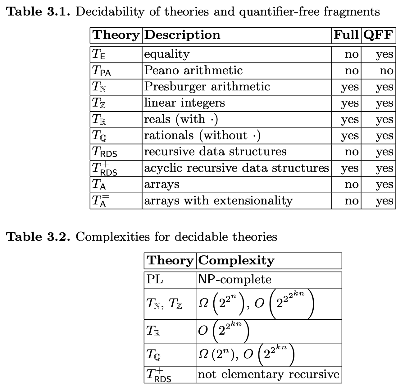
上述表格内的 Full 是指包含量词,而 QFF 指的是不包含量词。
## 程序正确性
对于计算机程序的正确性,我们分为两种: Partial correctness(也被称为 safety) 和 Total correctness(也被称为 progress)。Partial correctness 指断言(assert) 某些状态(一般指错误状态)在程序执行时不会出现,该结论的一个重要子集是: 假如一个程序具有 Partial correctness ,那么该程序如果可以 halt,那么 halt 后输出一定满足与输入的某种关系。此处注意 Partial correctness 并不要求程序一定可以 halt。而 Total correctness 刚好补充了这一点,Total correctness 要求在满足 Partial correctness 基础上,程序一定可以 halt。
对于 Partial correctness,我们一般使用一种被称为 inductive assertion method 的方法,该方法实际上基于递归证明程序的正确性,我们首先证明程序的初始状态就是满足预先给定的 FOL 表达式 $F$(即 base case),然后假设程序一直满足 $F$,证明在进行一步或者几步执行后,$F$ 仍被满足(即 inductive step)。假如我们希望进一步证明 Total correctness,那么我们就需要额外证明程序是可以停机的。此时我们会使用 ranking function method,这种方法会将程序内状态与一个函数(ranking function) 结合起来,接下来,我们使用 inductive assertion method 证明 ranking function 是在任何程序的状态转化下都是递减的。由于 ranking function 是递减的,那么程序最终会 halt。
### Annotations
Program Annotations 是形式化证明的核心。Program Annotations 是一个与程序内的变量有关的 FOL 表达式,我们可以认为 Program Annotations 就是一个我们对程序内变量在正确执行时需要满足约束的表达式。换言之,假如 annotations 不被满足,那么就说明程序内某些变量出现了我们未知的异常。后文所有代码内使用 `@` 开头的内容都是 annotations。从更加抽象的角度看,annotations 其实就是我们认为的代码不变量,无论代码如何执行,这些不变量不应该被打破。
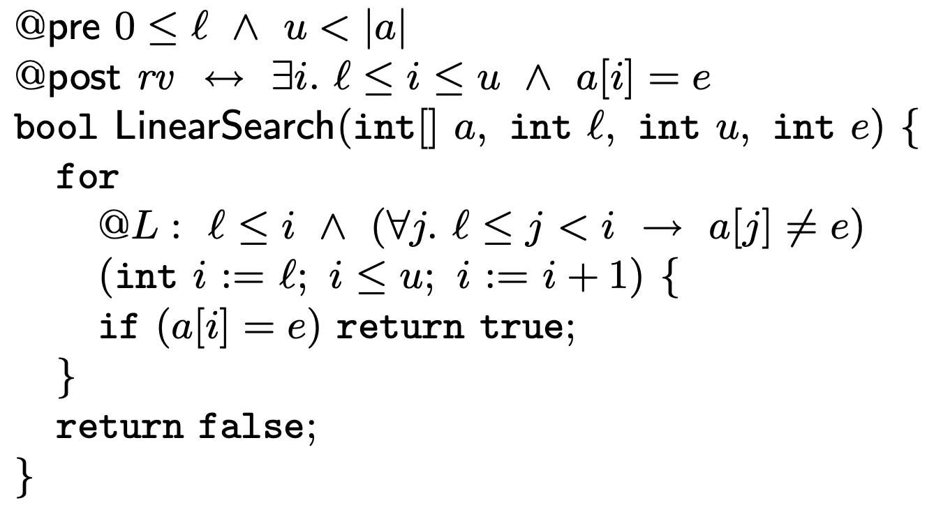
存在一种特殊的 Annotations 被称为 Function Specifications。对于任何在程序内定义的函数,函数都存在一对 annotations,分别为 function precondition 和 function postcondition,代表我们预期函数的入参满足的约束(在后文代码内使用 `@pre` 表示),以及函数输出 $rv$ 满足的约束(在后文代码内使用 `@post` 表示)。我们称 function precondition 和 function postcondition 为 Function Specifications。举一个简单例子,在数组的线性搜索中,我们可以给出如下 function specification:
```c
@pre 0 ≤ ℓ ∧ u < |a|
@post rv ↔ ∃i. ℓ ≤ i ≤ u ∧ a[i] = e
bool LinearSearch(int[] a, int ℓ, int u, int e) {
for (int i := ℓ; i ≤ u; i := i + 1) {
if (a[i] = e) return true;
}
return false;
}
```
上述代码内出现的 $0 \le \ell \land u < |a|$,实际上含义是线性搜索的起始位置 $\ell$ 应该大于 0 且线性搜索的结束位置 $u$ 小于数组 $a$ 的长度 $|a|$。而 $rv \leftrightarrow \exists i. \ell \le i \le u \land a[i] = e$ 是我们希望最终的输出结果 `rv` 需要满足的条件,其实就是要求线性搜索获得的 $i$ 位于 $\ell$ 和 $u$ 之间且搜索到的结果 $a[i]$ 与我们指定的输入 $e$ 相等。上述约束显然是不够稳健的,可以想象到 $u < \ell$ 也是符合 `@pre` 内的约束,但是显然这种终点小于起点的输入没有任何意义。对于 `LinearSearch` 一个更好的 annotations 如下:
$$
\begin{align*}
&@\text{pre}\ \ \top\\
&@\text{post}\ \ rv \leftrightarrow \exists i. 0 \le \ell \le i \le u < |a| \land a[i] = e
\end{align*}
$$
上述 `@pre` 等同于不对输入进行任何约束,而 `@post` 内结合代码最终结果对输入进行了额外约束。对于冒泡排序,我们可以给出如下的代码与 function specifications(原谅我此处直接给出图片而不是手动输入 latex):
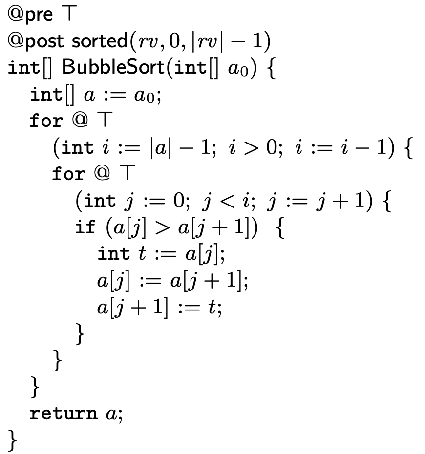 `@post` 内的 `sorted(a, l, u)` 是一个函数代表 `a` 列表从 `l` 到 `u` 的部分都已经进行了排序。实际上可以翻译为如下 FOL:
$$
\text{sorted}(a, l, u) \leftrightarrow (\forall i, j. l \le i \le j \le u \to a[i] \le a[j])
$$
可以在 smt2 内进行如下定义:
```lisp
(define-fun sorted ((arr (Array Int Int)) (l Int) (u Int)) Bool
(forall ((i Int) (j Int))
(=> (and (<= l i) (<= i j) (<= j u))
(<= (select arr i) (select arr j)))))
```
回到上述 BubbleSort 代码,由于我们从 `0` 开始进行数组的索引,所以数组的最后一个元素位于 $|rv| - 1$ 的位置。此处额外说明,上文展示的编程语言不会对输入进行任何更新,所以 BubbleSort 的第一行代码是将输入复制到内部变量中。至此,我们就完成了 Function Specifications 的初步学习,大部分形式化证明专用语言都会存在类似语法实现上述功能,比如 [Dafny](https://dafny.org/) 内的 `requires` 表示 `@pre` ,而 `ensures` 表示 `@post`。在 [Getting Started with Dafny: A Guide ](https://dafny.org/latest/%20OnlineTutorial/guide) 内存在以下示例代码:
```java
method Abs(x: int) returns (y: int)
ensures 0 <= y
{
if x < 0 {
return -x;
} else {
return x;
}
}
```
接下来,我们处理一些有趣的 annotations,首先介绍 Loop Invariants。这是用于 `while` 或者 `for` 循环的。对于 `while` 循环而言,我们可以看到如下片段:
$$
\begin{array}{l}
\texttt{while} \\
\quad @F \\
\quad (\langle \text{condition} \rangle) \{ \\
\quad \langle \text{body} \rangle \\
\}
\end{array}
$$
上述代码片段内的 `@F` 就是 loop invariant。我们可以看到我们额外标记的 $F$ 被插入到了每次 `condition` 评估前。在满足 $F \land \langle \text{condition} \rangle$ 情况下,我们会进入 `body` 代表的循环体,而在 $F \land \neg \langle \text{condition} \rangle$ 的条件下,我们会退出循环。考虑 `for` 循环:
$$
\begin{array}{l}
\texttt{for} \\
\quad @F \\
\quad (\langle \text{initialize} \rangle ;\langle \text{condition} \rangle; \langle \text{increment} \rangle) \{ \\
\quad \langle \text{body} \rangle \\
\}
\end{array}
$$
上述代码等同于以下 `while` 循环:
$$
\begin{array}{l}
\langle \text{initialize} \rangle \\
\texttt{while} \\
\quad @F \\
\quad (\langle \text{condition} \rangle) \{ \\
\quad \langle \text{body} \rangle \\
\quad \langle \text{increment} \rangle \\
\}
\end{array}
$$
在 `initialize` 后,我们要求 $F$ 必须成立,而且在每一次在 `condition` 评估前,$F$ 也必须成立。下图展示了 `LinearSearch` 的 Loop invariant `@L`:
`@post` 内的 `sorted(a, l, u)` 是一个函数代表 `a` 列表从 `l` 到 `u` 的部分都已经进行了排序。实际上可以翻译为如下 FOL:
$$
\text{sorted}(a, l, u) \leftrightarrow (\forall i, j. l \le i \le j \le u \to a[i] \le a[j])
$$
可以在 smt2 内进行如下定义:
```lisp
(define-fun sorted ((arr (Array Int Int)) (l Int) (u Int)) Bool
(forall ((i Int) (j Int))
(=> (and (<= l i) (<= i j) (<= j u))
(<= (select arr i) (select arr j)))))
```
回到上述 BubbleSort 代码,由于我们从 `0` 开始进行数组的索引,所以数组的最后一个元素位于 $|rv| - 1$ 的位置。此处额外说明,上文展示的编程语言不会对输入进行任何更新,所以 BubbleSort 的第一行代码是将输入复制到内部变量中。至此,我们就完成了 Function Specifications 的初步学习,大部分形式化证明专用语言都会存在类似语法实现上述功能,比如 [Dafny](https://dafny.org/) 内的 `requires` 表示 `@pre` ,而 `ensures` 表示 `@post`。在 [Getting Started with Dafny: A Guide ](https://dafny.org/latest/%20OnlineTutorial/guide) 内存在以下示例代码:
```java
method Abs(x: int) returns (y: int)
ensures 0 <= y
{
if x < 0 {
return -x;
} else {
return x;
}
}
```
接下来,我们处理一些有趣的 annotations,首先介绍 Loop Invariants。这是用于 `while` 或者 `for` 循环的。对于 `while` 循环而言,我们可以看到如下片段:
$$
\begin{array}{l}
\texttt{while} \\
\quad @F \\
\quad (\langle \text{condition} \rangle) \{ \\
\quad \langle \text{body} \rangle \\
\}
\end{array}
$$
上述代码片段内的 `@F` 就是 loop invariant。我们可以看到我们额外标记的 $F$ 被插入到了每次 `condition` 评估前。在满足 $F \land \langle \text{condition} \rangle$ 情况下,我们会进入 `body` 代表的循环体,而在 $F \land \neg \langle \text{condition} \rangle$ 的条件下,我们会退出循环。考虑 `for` 循环:
$$
\begin{array}{l}
\texttt{for} \\
\quad @F \\
\quad (\langle \text{initialize} \rangle ;\langle \text{condition} \rangle; \langle \text{increment} \rangle) \{ \\
\quad \langle \text{body} \rangle \\
\}
\end{array}
$$
上述代码等同于以下 `while` 循环:
$$
\begin{array}{l}
\langle \text{initialize} \rangle \\
\texttt{while} \\
\quad @F \\
\quad (\langle \text{condition} \rangle) \{ \\
\quad \langle \text{body} \rangle \\
\quad \langle \text{increment} \rangle \\
\}
\end{array}
$$
在 `initialize` 后,我们要求 $F$ 必须成立,而且在每一次在 `condition` 评估前,$F$ 也必须成立。下图展示了 `LinearSearch` 的 Loop invariant `@L`:
 在 Dafny 内,所有的循环也被要求使用 `invariant` 标注 loop invariant,具体可以参考 [Dafny Guide](https://dafny.org/latest/%20OnlineTutorial/guide) 内的 `Loop Invariants` 一节。
除了用于函数的 `@pre` 和 `@post` 与用于循环结构的 `@L` 外,我们也可以在任何代码前插入 annotation,这种 annotation 一般被称为 **assertion**,用于保证后续代码的正确性。比如我们可以在 `LinearSearch` 代码中的 `if (a[i] = e) return true;` 前插入 $0 \le i < |a|$ 以避免数组的越界访问。我们一般会将 assertion 分为两类:
1. 我们手动编写的作为 annotation 存在的 assertion。这些 assertion 会被用于后续的形式化证明
2. 编译器自动增加的 Runtime assertions,比如 Solidity 编译器默认会对所有数学计算进行溢出检查,一旦发现溢出,那么程序就会触发异常(runtime errors),还比如常见的传统语言编译器会保证的数组不会被越界访问等
在 dafny 内,我们可以使用 `assert 2 < 3;` 类似的语法进行断言,注意对数组的越界访问会默认插入越界访问的 `assert` 语句,。在 Solidity 的 SMTChecker 中,Solidity 编译器会将 `assert` 视为 annotation,有趣的是,`require` 语句内的内容会被视为始终成立的 `assumptions`,这会与我们后文讨论的一些内容有关。
在有了上述知识后,我们可以进行真正的形式化证明。我们的目标是证明 `LinearSearch` 算法的正确性。下图展示了包含所有 annotation 的 `LinearSearch` 代码(我们会在稍后的内容介绍 `BubbleSort` 的形式化证明,因为 BubbleSort 的 loop invariant 稍微复杂一些 )。在此处,我们再次给出 `LinearSearch` 的源代码:
对于任何代码的 partially correct 分为两步:
1. 将代码拆分为 basic paths,该步骤本质上是考虑代码的执行流,并将其拆分为几个不同的片段,在这里,我们需要注意 loop invariants 和 function specification 的作用
2. 将每一个 basic paths 转化为 verification conditions (VCs)。VC 是一个 FOL,所以我们只需要对 VC 进行 Satisfiability 检查即可
### Basic Path
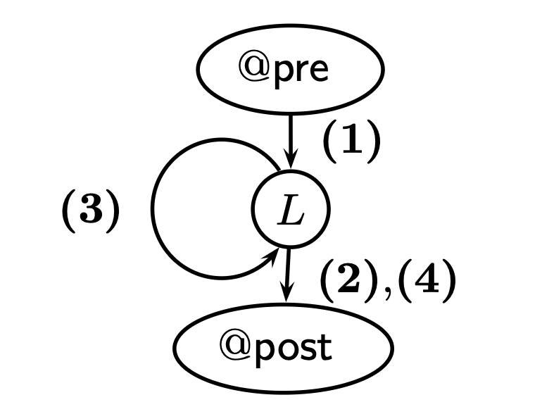
首先我们需要明确 basic path 是以 function pre-condition 或 loop invariant 作为起点,以 loop invariant / assertion 或者 function postcondition 作为终点的执行序列。对于 `LinearSearch` 而言,第 (1) 条 path 是以 `@pre` 开始到代表 loop invariant 的 `@L` 结束。注意,很多读者可以认为 basic path 是完整的代码执行流,从函数入口开始到函数返回结束,但是这种认识是错误的,实际上如上文所述,basic path 其实是对执行流的拆分。那么 path (1) 具体内容为:
$$
\begin{array}{l}
\text{@pre}\quad 0 \le \ell \land u < |a|\\
i := \ell;\\
\text{@L:}\quad \ell \le i \land (\forall j. \ell \le j < i \to a[j] \ne e)
\end{array}
$$
正如前文讨论的,对于 `for` 循环而言,`initialize` 语句会被视为在 loop invariant 前发生的。根据 basic path 的定义,后续所有的 path 都是在会以 `@L` 为开始,显然还存在三条 path:
1. $i \le u$ 成立,但是 `if` 判定中出现 $a[i] = e$ 成立,此时 path 的结束是 `@post`,即 `LinearSearch` 执行结束,记为 (2)
2. $i \le u$ 成立,但是 `if` 判定中出现 $a[i] \ne e$ 成立,此时 path 的结束是 `@L`,记为 (3)
3. $i > u$ 成立,`for` 循环判定失败被跳过,此时 path 的结束是 `@post`,记为 (4)
我们首先编写 path (2) 的情况:
$$
\begin{array}{l}
\text{@L:}\quad \ell \le i \land (\forall j. \ell \le j < i \to a[j] \ne e)\\
\text{assume} \quad i \le u;\\
\text{assume} \quad a[i] = e;\\
rv := \texttt{true};\\
\text{@post:}\quad rv \leftrightarrow \exists j. \ell \le j \le u \land a[j] = e
\end{array}
$$
此处,我们需要注意 `assume` 的语句,该语句表示这条 path 只会在 `assume` 成立下才会成立。换言之,我们可以将 assume statements 理解为 path 成立的前置条件。在 solidity 的 SMTChecker 中,`require` 就充当了 assume statements,但由于 `require` 本身也在代码内大量被使用抛出异常,所以部分基于 solidity 的形式化证明框架选择了其他的关键词以避免语义混淆,比如 [halmos](https://github.com/a16z/halmos/) 使用了 `vm.assume` 作为形式化证明下的 assume statements。dafny 内也存在 `assume` 语句,但是因为 dafny 自动完成了 path 的拆分和 path 对应的 VC 的验证,所以 `assume` 并不经常被使用,一般被用于大型形式化证明。而且使用 `assume` 会自动抛出警告,用户必须要将其手动修改为 `assume {:axiom}` 才可以抑制警告,避免用户出现误用的情况。
同理,我们可以得到 path (3) 的情况:
$$
\begin{array}{l}
\text{@L:}\quad \ell \le i \land (\forall j. \ell \le j < i \to a[j] \ne e)\\
\text{assume} \quad i \le u;\\
\text{assume} \quad a[i] \ne e;\\
i := i + 1;\\
\text{@L:}\quad \ell \le i \land (\forall j. \ell \le j < i \to a[j] \ne e)
\end{array}
$$
对于 path (4) 而言,最为简单:
$$
\begin{array}{l}
\text{@L:}\quad \ell \le i \land (\forall j. \ell \le j < i \to a[j] \ne e)\\
rv := \texttt{false};\\
\text{@post:}\quad rv \leftrightarrow \exists j. \ell \le j \le u \land a[j] = e
\end{array}
$$
对于 path (4) 而言,一定有读者好奇此处的 `@post` 是成立的吗?答案是肯定的,因为此时 `rv = false` 而 $\exists j. \ell \le j \le u \land a[j] = e $ 此时也是不成立。
我们可以使用下图表示 basic path 之间的关系,为了避免遗漏,我们一般使用深度优先(DFS)的方式逐条给出路径。
在 Dafny 内,所有的循环也被要求使用 `invariant` 标注 loop invariant,具体可以参考 [Dafny Guide](https://dafny.org/latest/%20OnlineTutorial/guide) 内的 `Loop Invariants` 一节。
除了用于函数的 `@pre` 和 `@post` 与用于循环结构的 `@L` 外,我们也可以在任何代码前插入 annotation,这种 annotation 一般被称为 **assertion**,用于保证后续代码的正确性。比如我们可以在 `LinearSearch` 代码中的 `if (a[i] = e) return true;` 前插入 $0 \le i < |a|$ 以避免数组的越界访问。我们一般会将 assertion 分为两类:
1. 我们手动编写的作为 annotation 存在的 assertion。这些 assertion 会被用于后续的形式化证明
2. 编译器自动增加的 Runtime assertions,比如 Solidity 编译器默认会对所有数学计算进行溢出检查,一旦发现溢出,那么程序就会触发异常(runtime errors),还比如常见的传统语言编译器会保证的数组不会被越界访问等
在 dafny 内,我们可以使用 `assert 2 < 3;` 类似的语法进行断言,注意对数组的越界访问会默认插入越界访问的 `assert` 语句,。在 Solidity 的 SMTChecker 中,Solidity 编译器会将 `assert` 视为 annotation,有趣的是,`require` 语句内的内容会被视为始终成立的 `assumptions`,这会与我们后文讨论的一些内容有关。
在有了上述知识后,我们可以进行真正的形式化证明。我们的目标是证明 `LinearSearch` 算法的正确性。下图展示了包含所有 annotation 的 `LinearSearch` 代码(我们会在稍后的内容介绍 `BubbleSort` 的形式化证明,因为 BubbleSort 的 loop invariant 稍微复杂一些 )。在此处,我们再次给出 `LinearSearch` 的源代码:
对于任何代码的 partially correct 分为两步:
1. 将代码拆分为 basic paths,该步骤本质上是考虑代码的执行流,并将其拆分为几个不同的片段,在这里,我们需要注意 loop invariants 和 function specification 的作用
2. 将每一个 basic paths 转化为 verification conditions (VCs)。VC 是一个 FOL,所以我们只需要对 VC 进行 Satisfiability 检查即可
### Basic Path
首先我们需要明确 basic path 是以 function pre-condition 或 loop invariant 作为起点,以 loop invariant / assertion 或者 function postcondition 作为终点的执行序列。对于 `LinearSearch` 而言,第 (1) 条 path 是以 `@pre` 开始到代表 loop invariant 的 `@L` 结束。注意,很多读者可以认为 basic path 是完整的代码执行流,从函数入口开始到函数返回结束,但是这种认识是错误的,实际上如上文所述,basic path 其实是对执行流的拆分。那么 path (1) 具体内容为:
$$
\begin{array}{l}
\text{@pre}\quad 0 \le \ell \land u < |a|\\
i := \ell;\\
\text{@L:}\quad \ell \le i \land (\forall j. \ell \le j < i \to a[j] \ne e)
\end{array}
$$
正如前文讨论的,对于 `for` 循环而言,`initialize` 语句会被视为在 loop invariant 前发生的。根据 basic path 的定义,后续所有的 path 都是在会以 `@L` 为开始,显然还存在三条 path:
1. $i \le u$ 成立,但是 `if` 判定中出现 $a[i] = e$ 成立,此时 path 的结束是 `@post`,即 `LinearSearch` 执行结束,记为 (2)
2. $i \le u$ 成立,但是 `if` 判定中出现 $a[i] \ne e$ 成立,此时 path 的结束是 `@L`,记为 (3)
3. $i > u$ 成立,`for` 循环判定失败被跳过,此时 path 的结束是 `@post`,记为 (4)
我们首先编写 path (2) 的情况:
$$
\begin{array}{l}
\text{@L:}\quad \ell \le i \land (\forall j. \ell \le j < i \to a[j] \ne e)\\
\text{assume} \quad i \le u;\\
\text{assume} \quad a[i] = e;\\
rv := \texttt{true};\\
\text{@post:}\quad rv \leftrightarrow \exists j. \ell \le j \le u \land a[j] = e
\end{array}
$$
此处,我们需要注意 `assume` 的语句,该语句表示这条 path 只会在 `assume` 成立下才会成立。换言之,我们可以将 assume statements 理解为 path 成立的前置条件。在 solidity 的 SMTChecker 中,`require` 就充当了 assume statements,但由于 `require` 本身也在代码内大量被使用抛出异常,所以部分基于 solidity 的形式化证明框架选择了其他的关键词以避免语义混淆,比如 [halmos](https://github.com/a16z/halmos/) 使用了 `vm.assume` 作为形式化证明下的 assume statements。dafny 内也存在 `assume` 语句,但是因为 dafny 自动完成了 path 的拆分和 path 对应的 VC 的验证,所以 `assume` 并不经常被使用,一般被用于大型形式化证明。而且使用 `assume` 会自动抛出警告,用户必须要将其手动修改为 `assume {:axiom}` 才可以抑制警告,避免用户出现误用的情况。
同理,我们可以得到 path (3) 的情况:
$$
\begin{array}{l}
\text{@L:}\quad \ell \le i \land (\forall j. \ell \le j < i \to a[j] \ne e)\\
\text{assume} \quad i \le u;\\
\text{assume} \quad a[i] \ne e;\\
i := i + 1;\\
\text{@L:}\quad \ell \le i \land (\forall j. \ell \le j < i \to a[j] \ne e)
\end{array}
$$
对于 path (4) 而言,最为简单:
$$
\begin{array}{l}
\text{@L:}\quad \ell \le i \land (\forall j. \ell \le j < i \to a[j] \ne e)\\
rv := \texttt{false};\\
\text{@post:}\quad rv \leftrightarrow \exists j. \ell \le j \le u \land a[j] = e
\end{array}
$$
对于 path (4) 而言,一定有读者好奇此处的 `@post` 是成立的吗?答案是肯定的,因为此时 `rv = false` 而 $\exists j. \ell \le j \le u \land a[j] = e $ 此时也是不成立。
我们可以使用下图表示 basic path 之间的关系,为了避免遗漏,我们一般使用深度优先(DFS)的方式逐条给出路径。
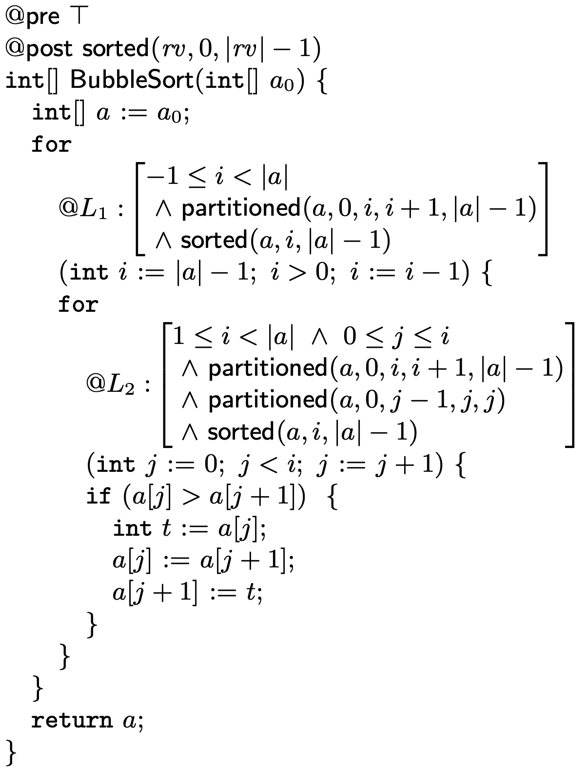
 对于 BubbleSorted 的 basic path 会更加复杂,我们在此展示 BubbleSorted 的原始代码:
我们可以看到此处包括两个 loop invariant,按照出现顺序,我们将其称为 $L_1$ 和 $L_2$。对于处于外层循环的 $L_1$ 而言,此时程序的状态应该是:
1. `i` 应该在区间 $[-1, |a| - 1]$ 内,其中在数组长度为 0 时,`i` 会被初始化为 -1
2. 数组 $a$ 的从 `i` 开始应该是已经完成排序的(即 $[i, |a| - 1]$ 的部分),正确实现的冒泡排序必然产生此结果
3. 冒泡排序由于每次都将未排序部分的最大数值向后移动,所以会出现 $[0, i]$ 部分内任一元素小于或等于 $[i+1, |a| - 1]$ 部分的任一元素,我们约定这种关系为 `partitioned`
`partitioned` 是一个定义如下的 predicate:
$$
\text{partitioned}(a, \ell_1, u_1, \ell_2, u_2) \iff \forall i,j. \ell_1 \le i \le u_1 < \ell_2 \le j \le u_2 \to a[i] \le a[j]
$$
对于 $L_2$ 而言,正确的程序应该满足如下状态:
1. $i$ 在区间 $[1, |a| - 1]$ 内,此处与 $L_1$ 的区间并不相同,这是因为 $L_1$ 状态经过 `for` 循环内的条件判断 $i > 0$ 后,在 $L_2$ 处已经不存在 $i = -1$ 或 $i = 0$ 的情况;$j$ 位于区间 $[0, i]$
2. 数组 $a$ 在 $[i, |a| - 1]$ 部分是完成排序的,这其实外层循环决定的
3. 数组 $a$ 的 partitioned 情况也与外层循环一致
4. 额外的,在 $[0, j -1]$ 部分的元素都小于或等于 $a[j]$,也可以使用 $\text{partitioned}(a, 0, j− 1, j, j)$ 表示
最后,带有完整 loop invariants 的代码如下:
对于 BubbleSorted 的 basic path 会更加复杂,我们在此展示 BubbleSorted 的原始代码:
我们可以看到此处包括两个 loop invariant,按照出现顺序,我们将其称为 $L_1$ 和 $L_2$。对于处于外层循环的 $L_1$ 而言,此时程序的状态应该是:
1. `i` 应该在区间 $[-1, |a| - 1]$ 内,其中在数组长度为 0 时,`i` 会被初始化为 -1
2. 数组 $a$ 的从 `i` 开始应该是已经完成排序的(即 $[i, |a| - 1]$ 的部分),正确实现的冒泡排序必然产生此结果
3. 冒泡排序由于每次都将未排序部分的最大数值向后移动,所以会出现 $[0, i]$ 部分内任一元素小于或等于 $[i+1, |a| - 1]$ 部分的任一元素,我们约定这种关系为 `partitioned`
`partitioned` 是一个定义如下的 predicate:
$$
\text{partitioned}(a, \ell_1, u_1, \ell_2, u_2) \iff \forall i,j. \ell_1 \le i \le u_1 < \ell_2 \le j \le u_2 \to a[i] \le a[j]
$$
对于 $L_2$ 而言,正确的程序应该满足如下状态:
1. $i$ 在区间 $[1, |a| - 1]$ 内,此处与 $L_1$ 的区间并不相同,这是因为 $L_1$ 状态经过 `for` 循环内的条件判断 $i > 0$ 后,在 $L_2$ 处已经不存在 $i = -1$ 或 $i = 0$ 的情况;$j$ 位于区间 $[0, i]$
2. 数组 $a$ 在 $[i, |a| - 1]$ 部分是完成排序的,这其实外层循环决定的
3. 数组 $a$ 的 partitioned 情况也与外层循环一致
4. 额外的,在 $[0, j -1]$ 部分的元素都小于或等于 $a[j]$,也可以使用 $\text{partitioned}(a, 0, j− 1, j, j)$ 表示
最后,带有完整 loop invariants 的代码如下:
 该部分展开的 basic path 路径较多,我们此处逐条给出,建议读者自己先尝试写一下,在核对笔者的答案:
Path (1) 是从 `@pre` 开始到 $L_1$ 结束:
$$
\begin{array}{l}
\text{@pre:}\quad \top\\
a := a_0;\\
i := |a| - 1;\\
\text{@}L_1\text{:}\quad -1 \le i < |a| \land \text{partitioned}(a, 0, i, i+1, |a| - 1) \land \text{sorted}(a, i, |a|-1)
\end{array}
$$
此处的 $i := |a| - 1$ 来自外层 `for` 循环的 `initialize` 语句。为了简化后续内容,我们将不再给出 $L_1$ 的完整内容。Path (2) 是从 $L_1$ 开始到 $L_2$ 结束:
$$
\begin{array}{l}
\text{@}L_1\\
\text{assume} \quad i > 0;\\
j := 0;\\
\text{@}L_2\text{:}\quad 1\le i < |a| \land 0 \le j \le i \land \text{partitioned}(a, 0, i, i +1, |a| - 1)\\
\quad \quad \quad \land \text{partitioned}(a, 0, j-1, j, j) \land \text{sorted}(a, i, |a|-1)\\
\end{array}
$$
此处的 `assume i > 0` 实际来自外层 `for` 循环内的 `i > 0` 的约束。为了简化,后文不再给出 $L_2$ 的完整表示。继续进行深度搜索,读者可能已经可以看到存在一条路径是 `j < i` 不成立导致无法进入内存循环到路径,但是该路径不是深度优先需要首先考虑的。根据深度优先的原则,我们首先考虑进入内层循环且内层循环内 `if` 成立时的 path (3)。该 path 从 $L_2$ 开始到 $L_2$ 结束:
$$
\begin{array}{l}
\text{@}L_2\\
\text{assume} \quad j < i;\\
\text{assume} \quad a[j] > a[j+1];\\
t := a[j];\\
a[j] := a[j+1];\\
a[j+1] := t;\\
j := j + 1;\\
\text{@}L_2
\end{array}
$$
接下来,考虑 `if` 循环不成立的情况 path (4):
$$
\begin{array}{l}
\text{@}L_2\\
\text{assume} \quad j < i;\\
\text{assume} \quad a[j] \le a[j+1];\\
j := j + 1;\\
\text{@}L_2
\end{array}
$$
接下来,我们才考虑刚刚提到但没有展示的由于 $j \ge i$ 而无法进入内层循环的情况 path (5):
$$
\begin{array}{l}
\text{@}L_2\\
\text{assume} \quad j \ge i;\\
i := i - 1;\\
\text{@}L_1
\end{array}
$$
以及最终从 $L_1$ 到 `@post` 到 path (6):
$$
\begin{array}{l}
\text{@}L_1\\
\text{assume} \quad i \le 0;\\
rv := a;\\
\text{@post} \quad \text{sorted}(rv, 0, |rv| - 1)
\end{array}
$$
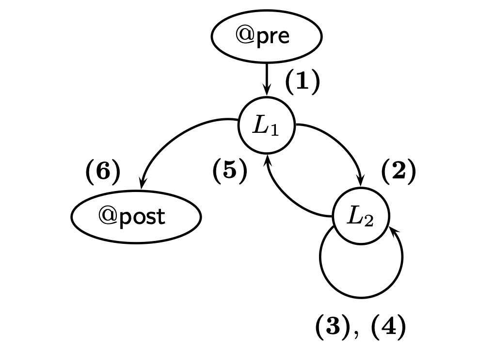
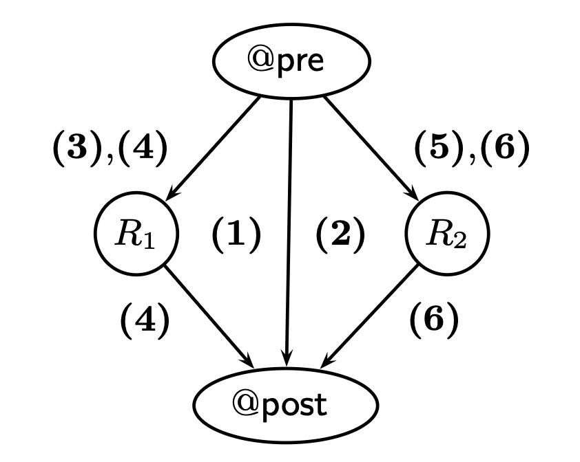
可视化展示所有的 path 如下:
该部分展开的 basic path 路径较多,我们此处逐条给出,建议读者自己先尝试写一下,在核对笔者的答案:
Path (1) 是从 `@pre` 开始到 $L_1$ 结束:
$$
\begin{array}{l}
\text{@pre:}\quad \top\\
a := a_0;\\
i := |a| - 1;\\
\text{@}L_1\text{:}\quad -1 \le i < |a| \land \text{partitioned}(a, 0, i, i+1, |a| - 1) \land \text{sorted}(a, i, |a|-1)
\end{array}
$$
此处的 $i := |a| - 1$ 来自外层 `for` 循环的 `initialize` 语句。为了简化后续内容,我们将不再给出 $L_1$ 的完整内容。Path (2) 是从 $L_1$ 开始到 $L_2$ 结束:
$$
\begin{array}{l}
\text{@}L_1\\
\text{assume} \quad i > 0;\\
j := 0;\\
\text{@}L_2\text{:}\quad 1\le i < |a| \land 0 \le j \le i \land \text{partitioned}(a, 0, i, i +1, |a| - 1)\\
\quad \quad \quad \land \text{partitioned}(a, 0, j-1, j, j) \land \text{sorted}(a, i, |a|-1)\\
\end{array}
$$
此处的 `assume i > 0` 实际来自外层 `for` 循环内的 `i > 0` 的约束。为了简化,后文不再给出 $L_2$ 的完整表示。继续进行深度搜索,读者可能已经可以看到存在一条路径是 `j < i` 不成立导致无法进入内存循环到路径,但是该路径不是深度优先需要首先考虑的。根据深度优先的原则,我们首先考虑进入内层循环且内层循环内 `if` 成立时的 path (3)。该 path 从 $L_2$ 开始到 $L_2$ 结束:
$$
\begin{array}{l}
\text{@}L_2\\
\text{assume} \quad j < i;\\
\text{assume} \quad a[j] > a[j+1];\\
t := a[j];\\
a[j] := a[j+1];\\
a[j+1] := t;\\
j := j + 1;\\
\text{@}L_2
\end{array}
$$
接下来,考虑 `if` 循环不成立的情况 path (4):
$$
\begin{array}{l}
\text{@}L_2\\
\text{assume} \quad j < i;\\
\text{assume} \quad a[j] \le a[j+1];\\
j := j + 1;\\
\text{@}L_2
\end{array}
$$
接下来,我们才考虑刚刚提到但没有展示的由于 $j \ge i$ 而无法进入内层循环的情况 path (5):
$$
\begin{array}{l}
\text{@}L_2\\
\text{assume} \quad j \ge i;\\
i := i - 1;\\
\text{@}L_1
\end{array}
$$
以及最终从 $L_1$ 到 `@post` 到 path (6):
$$
\begin{array}{l}
\text{@}L_1\\
\text{assume} \quad i \le 0;\\
rv := a;\\
\text{@post} \quad \text{sorted}(rv, 0, |rv| - 1)
\end{array}
$$
可视化展示所有的 path 如下:
 在上文中,我们始终没有处理带有函数调用的情况。在二分查找算法内,我们会使用递归方法进行调用自身实现二分查找,对于这种包含函数调用的情况,我们该如何编写 basic path?
在前文中,我们介绍了 Function Specifications 内的 `@pre` 和 `@post` 。在面对函数调用时,我们会直接使用 `@post` 即函数输出替换掉函数调用。我们考虑函数 `f` 具有以下定义:
$$
\begin{array}{l}
\text{@pre}\quad F[p_1, \dots, p_n]\\
\text{@post}\quad G[p_1, \dots, p_n, rv]\\
f(p_1, \dots, p_n)
\end{array}
$$
假如我们在上下文中调用了 `f`:
$$
w := f(e_1, \dots, e_n)
$$
我们会首先在调用前增加 function call assertion 来保证输入参数是满足函数要求的:
$$
\begin{array}{l}
\dots\\
\text{@} F[e_1, \dots,e_n];\\
w := f(e_1, \dots, e_n);
\end{array}
$$
然后使用 assume 将函数的 `@post` 放入调用上下文,我们一般会引入一个新的变量代表函数返回值,然后将新的变量赋值给 `w`,如下:
$$
\begin{array}{l}
\dots\\
\text{@} F[e_1, \dots,e_n];\\
\text{assume}\ G[e1, . . . , en, v];\\
w := v;
\end{array}
$$
我们可以看到,对于代码内调用的外部函数,我们不在意外部函数的具体实现,而只在意外部函数的 `@post` 输出。在 Dafny 的 [入门教程](https://dafny.org/latest/%20OnlineTutorial/guide) 中,读者会读到以下内容:
> The reason this happens is that Dafny “forgets” about the body of every method except the one it is currently working on. This simplifies Dafny’s job tremendously, and is one of the reasons it is able to operate at reasonable speeds. It also helps us reason about our programs by breaking them apart and so we can analyze each method in isolation (given the annotations for the other methods).
上述内容中描述的 **forgets** 行为其实就是指在处理外部函数时,我们不会使用外部函数的具体实现,而只使用 `@post`。这意味着,假如开发者无法给出明确的且约束合适的对某个函数 `@post` 注解,那么可能会出现调用该函数的其他函数无法获得正确证明,比如 dafny 内的如下例子:
```java
method Abs(x: int) returns (y: int)
ensures 0 <= y
{
if x < 0 {
return -x;
} else {
return x;
}
}
method Testing()
{
var v := Abs(3);
assert 0 <= v;
assert v == 3;
}
```
由于此处的 `Abs` 使用 `0 <= y` 条件没有有效约束输出,这导致 `Testing` 无法被证明。正确的对 `Abs` 的 `@post` 约束如下:
```java
method Abs(x: int) returns (y: int)
ensures 0 <= y
ensures 0 <= x ==> y == x
ensures x < 0 ==> y == -x
{
if x < 0 {
return -x;
} else {
return x;
}
}
```
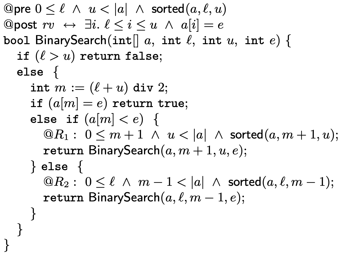
在积累上述知识后,我们回头看 BinarySearch 的 basic path。为了方便读者阅读,此处再次给出 BinarySearch 的源代码:

path (1) 是从 `@pre` 开始到第一个 `if` 分支出现 $\ell > u$ 而立即返回的情况:
$$
\begin{array}{l}
\text{@pre}\quad 0 \le \ell \land u < |a| \land \text{sorted}(a, \ell, u)\\
\text{assume}\quad \ell > u;\\
rv := \text{false};\\
\text{@post}\quad rv \iff \exists i. \ell \le i \le u \land a[i] = e
\end{array}
$$
path (2) 是从 `@pre` 开始到第二个 `if` 分支出现 `a[m] = e` 而立即返回的情况:
$$
\begin{array}{l}
\text{@pre}\quad 0 \le \ell \land u < |a| \land \text{sorted}(a, \ell, u)\\
\text{assume}\quad \ell \le u;\\
m := (\ell + u)\ \text{div}\ 2;\\
\text{assume}\quad a[m] = e; \\
rv := \text{true};\\
\text{@post}\quad rv \iff \exists i. \ell \le i \le u \land a[i] = e
\end{array}
$$
path (3) 是从 `@pre` 开始到 $R_1$ 结束的情况:
$$
\begin{array}{l}
\text{@pre}\quad 0 \le \ell \land u < |a| \land \text{sorted}(a, \ell, u)\\
\text{assume}\quad \ell \le u;\\
m := (\ell + u)\ \text{div}\ 2;\\
\text{assume}\quad a[m] \ne e; \\
\text{assume}\quad a[m] < e; \\
\text{@R}_1\quad 0 \le m + 1 \land u < |a| \land \text{sorted}(a, m+1, u)
\end{array}
$$
然后就是本节介绍的重点,我们需要在 path (4) 内完成函数调用:
$$
\begin{array}{l}
\text{@pre}\quad 0 \le \ell \land u < |a| \land \text{sorted}(a, \ell, u)\\
\text{assume}\quad \ell \le u;\\
m := (\ell + u)\ \text{div}\ 2;\\
\text{assume}\quad a[m] \ne e; \\
\text{assume}\quad a[m] < e; \\
\text{assume}\quad v_1 \iff \exists i. m+1 \le i \le u \land a[i] = e; \\
rv := v_1;\\
\text{@post}\quad rv \iff \exists i. \ell \le i \le u \land a[i] = e
\end{array}
$$
我们此处没有对输入的 $m+1$ 参数进行显性的约束,实际上根据 `@pre` 等约束条件可以很容易推导出 `m + 1` 是满足入参条件的。对于另一个 `if` 分支 $R_2$ 的情况,读者可以自行编写,最终我们可以获得 6 条 basic path。
在上文中,我们始终没有处理带有函数调用的情况。在二分查找算法内,我们会使用递归方法进行调用自身实现二分查找,对于这种包含函数调用的情况,我们该如何编写 basic path?

在前文中,我们介绍了 Function Specifications 内的 `@pre` 和 `@post` 。在面对函数调用时,我们会直接使用 `@post` 即函数输出替换掉函数调用。我们考虑函数 `f` 具有以下定义:
$$
\begin{array}{l}
\text{@pre}\quad F[p_1, \dots, p_n]\\
\text{@post}\quad G[p_1, \dots, p_n, rv]\\
f(p_1, \dots, p_n)
\end{array}
$$
假如我们在上下文中调用了 `f`:
$$
w := f(e_1, \dots, e_n)
$$
我们会首先在调用前增加 function call assertion 来保证输入参数是满足函数要求的:
$$
\begin{array}{l}
\dots\\
\text{@} F[e_1, \dots,e_n];\\
w := f(e_1, \dots, e_n);
\end{array}
$$
然后使用 assume 将函数的 `@post` 放入调用上下文,我们一般会引入一个新的变量代表函数返回值,然后将新的变量赋值给 `w`,如下:
$$
\begin{array}{l}
\dots\\
\text{@} F[e_1, \dots,e_n];\\
\text{assume}\ G[e1, . . . , en, v];\\
w := v;
\end{array}
$$
我们可以看到,对于代码内调用的外部函数,我们不在意外部函数的具体实现,而只在意外部函数的 `@post` 输出。在 Dafny 的 [入门教程](https://dafny.org/latest/%20OnlineTutorial/guide) 中,读者会读到以下内容:
> The reason this happens is that Dafny “forgets” about the body of every method except the one it is currently working on. This simplifies Dafny’s job tremendously, and is one of the reasons it is able to operate at reasonable speeds. It also helps us reason about our programs by breaking them apart and so we can analyze each method in isolation (given the annotations for the other methods).
上述内容中描述的 **forgets** 行为其实就是指在处理外部函数时,我们不会使用外部函数的具体实现,而只使用 `@post`。这意味着,假如开发者无法给出明确的且约束合适的对某个函数 `@post` 注解,那么可能会出现调用该函数的其他函数无法获得正确证明,比如 dafny 内的如下例子:
```java
method Abs(x: int) returns (y: int)
ensures 0 <= y
{
if x < 0 {
return -x;
} else {
return x;
}
}
method Testing()
{
var v := Abs(3);
assert 0 <= v;
assert v == 3;
}
```
由于此处的 `Abs` 使用 `0 <= y` 条件没有有效约束输出,这导致 `Testing` 无法被证明。正确的对 `Abs` 的 `@post` 约束如下:
```java
method Abs(x: int) returns (y: int)
ensures 0 <= y
ensures 0 <= x ==> y == x
ensures x < 0 ==> y == -x
{
if x < 0 {
return -x;
} else {
return x;
}
}
```
在积累上述知识后,我们回头看 BinarySearch 的 basic path。为了方便读者阅读,此处再次给出 BinarySearch 的源代码:

path (1) 是从 `@pre` 开始到第一个 `if` 分支出现 $\ell > u$ 而立即返回的情况:
$$
\begin{array}{l}
\text{@pre}\quad 0 \le \ell \land u < |a| \land \text{sorted}(a, \ell, u)\\
\text{assume}\quad \ell > u;\\
rv := \text{false};\\
\text{@post}\quad rv \iff \exists i. \ell \le i \le u \land a[i] = e
\end{array}
$$
path (2) 是从 `@pre` 开始到第二个 `if` 分支出现 `a[m] = e` 而立即返回的情况:
$$
\begin{array}{l}
\text{@pre}\quad 0 \le \ell \land u < |a| \land \text{sorted}(a, \ell, u)\\
\text{assume}\quad \ell \le u;\\
m := (\ell + u)\ \text{div}\ 2;\\
\text{assume}\quad a[m] = e; \\
rv := \text{true};\\
\text{@post}\quad rv \iff \exists i. \ell \le i \le u \land a[i] = e
\end{array}
$$
path (3) 是从 `@pre` 开始到 $R_1$ 结束的情况:
$$
\begin{array}{l}
\text{@pre}\quad 0 \le \ell \land u < |a| \land \text{sorted}(a, \ell, u)\\
\text{assume}\quad \ell \le u;\\
m := (\ell + u)\ \text{div}\ 2;\\
\text{assume}\quad a[m] \ne e; \\
\text{assume}\quad a[m] < e; \\
\text{@R}_1\quad 0 \le m + 1 \land u < |a| \land \text{sorted}(a, m+1, u)
\end{array}
$$
然后就是本节介绍的重点,我们需要在 path (4) 内完成函数调用:
$$
\begin{array}{l}
\text{@pre}\quad 0 \le \ell \land u < |a| \land \text{sorted}(a, \ell, u)\\
\text{assume}\quad \ell \le u;\\
m := (\ell + u)\ \text{div}\ 2;\\
\text{assume}\quad a[m] \ne e; \\
\text{assume}\quad a[m] < e; \\
\text{assume}\quad v_1 \iff \exists i. m+1 \le i \le u \land a[i] = e; \\
rv := v_1;\\
\text{@post}\quad rv \iff \exists i. \ell \le i \le u \land a[i] = e
\end{array}
$$
我们此处没有对输入的 $m+1$ 参数进行显性的约束,实际上根据 `@pre` 等约束条件可以很容易推导出 `m + 1` 是满足入参条件的。对于另一个 `if` 分支 $R_2$ 的情况,读者可以自行编写,最终我们可以获得 6 条 basic path。
 ## Verification Conditions
在上一节中,我们介绍了如何获得一段代码的 path,我们可以看到每一段 path 都是存在开始状态、动作和结束状态,我们一般使用 *Hoare triple* 表示:
$$
\{F\}S_1;\dots;S_n\{G\}
$$
我们需要证明在初始状态 $F$ 的情况下,经过 $S_1; \dots; S_n$ 语句操作后,最终获得的状态为 $G$。在具体的证明过程中,我们会使用被称为 weakest precondition 的机制。
weakest precondition $\mathrm{wp}(F,S)$ ,此处的 $F$ 指的是任意 FOL 表达式,而 $S$ 指程序语句。wp 的定义为如果程序状态 s 满足 $s \models \mathrm{wp}(F, S)$ 且此处的 $S$ 语句在状态 $s$ 操作后获得的状态 $s'$ 满足 $s' \models F$。换言之,假如结束状态满足 $F$,那么其前一个状态是满足 $\mathrm{wp}(F,S)$ 的。我们可以发现 $\mathrm{wp}(F,S)$ 提供了一种方法,允许我们将对 $\{F\}S_1;\dots;S_n\{G\}$ 的 correctness 证明转化为对单一命题的证明,方法是进行进行类似如下的调用:
$$
\mathrm{wp}(\mathrm{wp}(\mathrm{wp}(\mathrm{wp}(G, S_n), S_{n-1}), \dots),F)
$$
根据 wp 的定义,假如上述 FOL 是 valid 的,那么就意味着程序在任意状态下都是正确的。假如读者无法理解上述描述,也可以继续阅读,因为实际上无法理解原理也可以使用 wp 方法证明程序的正确性。
对于 Assumption 和 Assignment 语句而言,定义 wp 为:
1. $\mathrm{wp}(F, \text{assume } c) \iff c \to F$
2. $\mathrm{wp}(F[v], v:= e) \iff F[e]$,该表达式含义是将命题 $F$ 内的变量 $v$ 替换为 $e$,命题仍成立
对于一系列语句 $S_1; \dots; S_n$ ,我们定义:
$$
\mathrm{wp}(F, S_1; \dots; S_n) \iff \mathrm{wp}(\mathrm{wp}(F, S_n), S_1; \dots, S_{n-1})
$$
简单来说,我们会按照从后到前的顺序依次使用语句 $S$ 调用 wp 函数,此处的定义与上文的分析是一致的。对任意 basic path $\{F\}S_1;\dots;S_n\{G\}$ 而言,其 verification condition 为:
$$
F \to \mathrm{wp}(G, S_1, \dots, S_n)
$$
实际上我们只需要证明上述 verification condition 的 valid 属性,就可以证明对应的 basic path 的正确性。上述 verification condition 其实与 $\mathrm{wp}(\mathrm{wp}(\mathrm{wp}(\mathrm{wp}(G, S_n), S_{n-1}), \dots),F)$ 是一致的,我们只是将最终的 $\mathrm{wp}(\dots, F)$ 利用 Assumption 语句展开为了 $F \to \mathrm{wp}(G, S_1, \dots, S_n)$。
举例说明,以下 path 来自LinearSearch 的 path (2):
$$
\begin{array}{l}
\text{@F:}\quad \ell \le i \land (\forall j. \ell \le j < i \to a[j] \ne e)\\
S_1\text{ : }\texttt{assume } i \le u;\\
S_2\text{ : }\texttt{assume } a[i] = e;\\
S_3\text{ : }rv := \texttt{true};\\
\text{@post G:}\quad rv \leftrightarrow \exists j. \ell \le j \le u \land a[j] = e
\end{array}
$$
上述代码的 VC 是 $F \to \mathrm{wp}(G, S_1; S_2; S_3)$,我们首先计算 wp 函数部分:
$$
\begin{align*}
\mathrm{wp}&(G, S_1; S_2; S_3)\\
&\iff \mathrm{wp}(\mathrm{wp}(rv \leftrightarrow \exists j. \ell \le j \le u \land a[j] = e , rv := \texttt{true}), S_1; S_2)\\
&\iff \mathrm{wp}(\texttt{true} \leftrightarrow \exists j. \ell \le j \le u \land a[j] = e, S_1;S_2)\\
&\iff \mathrm{wp}(\exists j. \ell \le j \le u \land a[j] = e, S_1;S_2)\\
&\iff \mathrm{wp}(\mathrm{wp}(\exists j. \ell \le j \le u \land a[j] = e, \texttt{assume } a[i] = e), S_1)\\
&\iff \mathrm{wp}(a[i] = e \to \exists j. \ell \le j \le u \land a[j] = e, S_1)\\
&\iff \mathrm{wp}(a[i] = e \to \exists j. \ell \le j \le u \land a[j] = e, \texttt{assume } i \le u)\\
&\iff i\le u \to (a[i] = e \to \exists j. \ell \le j \le u \land a[j] = e)
\end{align*}
$$
完整的 VC 应该是:
$$
\begin{align*}
\ell &\le i \land (\forall j. \ell \le j < i \to a[j] \ne e)\\
& \to i\le u \to (a[i] = e \to \exists j. \ell \le j \le u \land a[j] = e)
\end{align*}
$$
在本文最开始,我们证明过 $F: A \to B \to C \iff (A \land B) \to C$,该命题的泛化版本是:
$$
F_1 \to F_2 \to \dots \to F_n \iff (F_1 \land \dots \land F_{n-1}) \to F_n
$$
所以上述 VC 可以被转化为:
$$
\begin{align*}
\ell &\le i \land (\forall j. \ell \le j < i \to a[j] \ne e) \\
& \land i\le u \land a[i] = e \to (\exists j. \ell \le j \le u \land a[j] = e)
\end{align*}
$$
读者可以直接把这个命题丢给 LLM 处理,此处笔者将上述命题丢给了 ChatGPT 处理获得了如下 smt2 代码:
```lisp
(set-logic AUFLIA)
(declare-sort Elem 0)
(declare-const l Int)
(declare-const i Int)
(declare-const u Int)
(declare-const e Elem)
(declare-const a (Array Int Elem))
(define-fun F () Bool
(=> (and
(<= l i)
(forall ((j Int))
(=> (and (<= l j) (< j i))
(not (= (select a j) e))))
(<= i u)
(= (select a i) e))
(exists ((j Int))
(and (<= l j)
(<= j u)
(= (select a j) e)))))
(assert (not F))
(check-sat)
```
输出结果应该是 `unsat`,说明 VC 是 valid 的,也可以证明 LinearSearch 的部分正确性,完全的正确性需要证明所有的 path 对应的 VC 都是 valid 的。后续的文章中,我们不会处理 VC 最终的证明,读者可以直接丢给 LLM 处理为 smt2 语言,然后由 z3 或者任何其他求解器处理。
我们可以看一个稍微有一点复杂的,BinarySearch 内的 path (2):
$$
\begin{array}{l}
\text{@pre F}\quad 0 \le \ell \land u < |a| \land \text{sorted}(a, \ell, u)\\
S_1\text{ : }\texttt{assume}\quad \ell \le u;\\
S_2\text{ : }m := (\ell + u)\ \texttt{div}\ 2;\\
S_3\text{ : }\texttt{assume}\quad a[m] = e; \\
S_4\text{ : }rv := \texttt{true};\\
\text{@post G}\quad rv \iff \exists i. \ell \le i \le u \land a[i] = e
\end{array}
$$
还是首先计算 $\mathrm{wp}(G, S_1; S_2; S_3; S_4)$ 部分:
$$
\begin{align*}
\mathrm{wp}&(G, S_1; S_2; S_3; S_4)\\
&\iff \mathrm{wp}(\mathrm{wp}(G, S_4), S_1; S_2; S_3)\\
&\iff \mathrm{wp}(\mathrm{wp}(G, rv := \texttt{true}), S_1; S_2; S_3)\\
&\iff \mathrm{wp}(\mathrm{wp}(G\{rv \mapsto \texttt{true}\}), S_1; S_2; S_3)\\
&\iff \mathrm{wp}(\mathrm{wp}(G\{rv \mapsto \texttt{true}\}, S_3), S_1; S_2)\\
&\iff \mathrm{wp}(\mathrm{wp}(G\{rv \mapsto \texttt{true}\}, \texttt{assume }a[m] = e), S_1; S_2)\\
&\iff \mathrm{wp}(a[m] = e \to G\{rv \mapsto \texttt{true}\}, S_1; S_2)\\
&\iff \mathrm{wp}(\mathrm{wp}(a[m] = e \to G\{rv \mapsto \texttt{true}\}, S_2), S_1)\\
&\iff \mathrm{wp}(\mathrm{wp}(a[m] = e \to G\{rv \mapsto \texttt{true}\}, m := (\ell + u)\ \texttt{div}\ 2), S_1)\\
&\iff \mathrm{wp}((a[m] = e \to G\{rv \mapsto \texttt{true}\})\{m \mapsto (\ell + u)\ \texttt{div}\ 2\}, S_1)\\
&\iff \mathrm{wp}((a[m] = e \to G\{rv \mapsto \texttt{true}\})\{m \mapsto (\ell + u)\ \texttt{div}\ 2\}, \texttt{assume } \ell \le u)\\
&\iff \ell \le u \to (a[m] = e \to G\{rv \mapsto \texttt{true}\})\{m \mapsto (\ell + u)\ \texttt{div}\ 2\}\\
&\iff \ell \le u \to (a[m] = e) \{m \mapsto (\ell + u)\ \texttt{div}\ 2\} \to G\{rv \mapsto \texttt{true}, m \mapsto (\ell + u)\ \texttt{div}\ 2\}\\
&\iff \ell \le u \to a[(\ell + u)\ \texttt{div}\ 2] = e \to G\{rv \mapsto \texttt{true}, m \mapsto (\ell + u)\ \texttt{div}\ 2\}\\
&\iff \ell \le u \to a[(\ell + u)\ \texttt{div}\ 2] = e \to \exists i. \ell \le i \le u \land a[i] = e
\end{align*}
$$
上述化简的最后 3 步都是在处理赋值问题,其实只需要将变量名对应的值带入 FOL 即可,假如该变量名不存在,比如 $G$ 中不存在 $m$ 变量,那么就可以忽略。
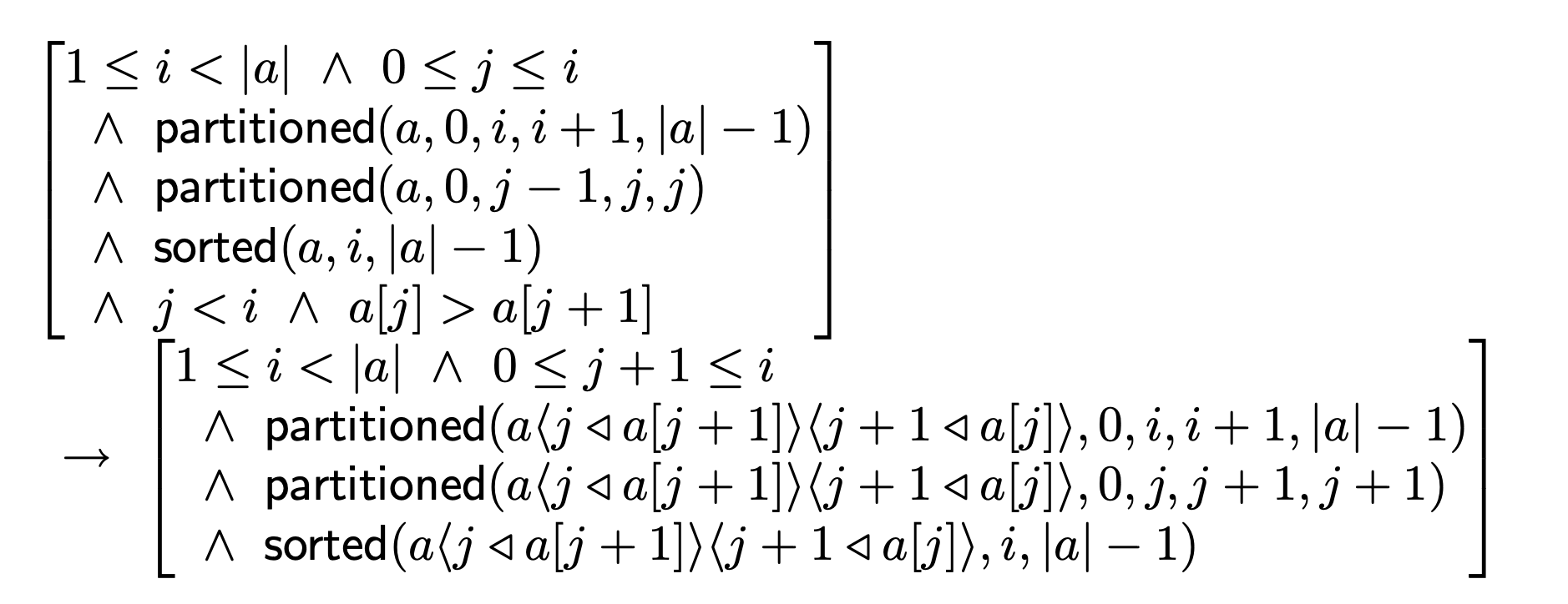
BubbleSort 的 path (3) 是一个相当复杂的案例,我们在此处只给出最终的结果:
## Total Correctness
在上一节中,我们介绍了如何使用基于 wp 的 VC 机制证明程序的 Partial correctness 属性,利用上述方法可以证明程序的 basic path 正确性,更加严谨来说,上述方法可以证明程序的任意状态都是符合我们预期的,但是上述方法无法证明程序会停机。在本节中,我们主要提供一种使用 ranking function 的方法。
在介绍具体的方法前,我们需要补充一个背景知识,即 *well-founded relation*。假设在集合 $S$ 上存在一个 binary predicate $\prec$ ,我们称 $\prec$ 是 well-founded relation 在有且仅有 $S$ 集合 **不存在** 无限长的序列 $s_1, s_2, \dots$ 满足 successive element 小于 predecessor:
$$
s_1 \succ s_2 \succ s_3 \succ \dots
$$
并且上述关系中存在 $s \succ t \iff t \prec s$。换言之,well-founded relation 要求集合 $S$ 内对 $\prec$ 关系只存在有限长度的序列。我们举例说明,对于自然数上的 $<$ 而言,$<$ 关系是满足 well-founded relation,因为任意的自然数序列在递减到 0 后就停止了,所以不存在基于 $<$ 构造的无限长度序列。但是在有理数集合内,$<$ 关系不是 well-founded relation,因为有理数集合可以出现以下递减序列:
$$
1 > \frac{1}{2} > \frac{1}{3} > \frac{1}{4} > \dots
$$
我们可以在有理数集合内可以构造出无限长的递减序列,所以有理数内的 $<$ 不是 well-founded relation。基于 well-founded relation,我们会用到一个派生概念 lexicographic relations。假设存在多个具有 well-founded relation 定义的集合的 $(S_1, \prec_1), (S_2, \prec_2), \dots, (S_m, \prec_m)$,基于此我们构建一个大的集合:
$$
S = S_1 \times \dots \times S_m
$$
对于 $s_i, t_i \in S_i$ ,定义以下 relation $\prec$
$$
(s_1, \ldots, s_m) \prec (t_1, \ldots, t_m)
\iff
\bigvee_{i=1}^{m}
\left(
s_i \prec_i t_i
\,\land\,
\bigwedge_{j=1}^{i-1} s_j = t_j
\right)
$$
上述 relation 的本质是对于元组 $s, t$ 内的元素进行逐一比较,直到找到第一个存在 $\prec$ 关系的元素,比如假设 $s = (3, 9, 10)$ 而 $t = (3, 11, 0)$,我们首先比较发现 $s_1 = t_1$,然后比较 $s_2 < t_2$,此时发现第一个满足 $\prec$ 的元素,那么 $s \prec t$ 是成立的,注意我们不关心 $s_3, t_3$ 的大小关系。对于这种自然数元组的 lexicographic 关系,我们通常使用 $<_n$ 表示,其中 $n$ 代表比较元组的长度,比如刚刚的示例其实就是 $<_3$
很多读者可能知道数学归纳法,对于自然数 $x$ 内的命题 $F[x]$ 标准的数学归纳法为:
1. base case: 证明 $F[0]$ 是 valid 的
2. inductive step: **假设**对于任意自然数 $n$,$F[n]$ 是 valid 的(即 inductive hypothesis,或缩写为 IH),我们需要证明 $F[n + 1]$ 也是 valid
当我们完成上述步骤后,我们就可以证明 $F[x]$ 对所有的自然数 $x$ 都是 valid 的。数学归纳法成立的原因是在自然数 $T_{\mathrm{PA}}$ 内存在以下公理(这个公理在本文开始介绍 theory 时也有出现):
$$
F[0] \land (\forall n. F[n] \to F[n+1]) \to \forall x. F[x]
$$
与之等价的还有另一种更加紧凑的表达递归过程公理的命题模版,如下:
$$
(\forall n. (\forall n'. n' < n \to F[n']) \to F[n]) \to \forall x. F[x]
$$
首先,此处的 inductive hypothesis 是对于任意自然数 $n$,已知 $n' < n$ 下,$F[n']$ 是 valid 的,我们需要在上述假设(即 $\forall n'. n' < n \to F[n']$) 基础上,证明 $F[n]$ 也是 valid。由于上述公理的存在,那么 $\forall x. F[x]$ 自然也是 valid 的。
上述命题实际上只表示了递归中的 inductive step 而没有包含 base case。但在很多情况下,base case 是隐含的,但有时候需要单独证明 $F[0]$ 的 valid 属性。比如在自然数情况下,不存在 $n' < 0$ 的情况,这说明 inductive step 没有隐含 base case ,所以需要单独证明 $F[0]$ 的 valid 属性。
举例说明,我们在自然数内引入如下两条与余数(remainder)有关的定理:
$$
\begin{array}{l}
\forall x,y. x < y \to rem(x,y) = x\\
\forall x, y. y > 0 \to rem(x + y, y) = rem(x, y)
\end{array}
$$
举一个具体数值计算 $rem(5, 3) = 2$。我们希望证明 $\forall y > 0 \to rem(x, y) < y$,即余数(remainder)总是小于除数(divisor)。
首先,我们可以直接给出 inductive hypothesis,此处我们选择对 $x$ 进行归纳,即对于任意的 $x$ 都存在(以下将 $n$ 替换为 $x$ 以及将 $n'$ 替换为 $x'$ 的操作是有一定危险的,因为 FOL 内存在量词约束变量,具体的安全替换方法可以参考参考书的 **2.4.1 Safe Substitution**)
$$
\forall y. y > 0 \to \forall x.((\forall x'. x' < x \to rem(x', y) < y) \to rem(x, y) < y)
$$
假如我们可以证明 $\forall x.((\forall x'. x' < x \to rem(x', y) < y) \to rem(x, y) < y)$ 是 valid 的,那么就可以证明 $\forall y. y > 0 \to \forall x. rem(x, y) < y$,这与我们希望证明的命题其实是等价的。对于形如 $H \to G$ 的待证明的命题,最简单的使用 $H$ 作为已知条件,对 $G$ 进行约化。
当然,此处存在两种情况 $x < y$ 以及 $\neg(x < y)$。对于 $x < y$ 的情况,我们有:
$$
rem(x, y) = x < y
$$
调用 $\forall x,y. x < y \to rem(x,y) = x$ 公理不难获得上述结论。对于 $\neg(x < y)$ 的情况,我们取 $x' = x - y$可以获得:
$$
rem(x, y) = rem(x', y) < y
$$
此处 $rem(x', y) < y$ 来自 inductive hypothesis。至此,我们证明了命题的 valid,也意味着最初的 $\forall y > 0 \to rem(x, y) < y$ 是 valid 的。
此处我们将本节最初介绍的 well-founded relation 引入,实际上 well-founded relation 和派生的 lexicographic relations 也可以进行归纳,这种归纳方法被称为 Well-founded induction,可以使用如下模版表示:
$$
(\forall n. (\forall n'. n' \prec n \to F[n']) \to F[n]) \to \forall x. F[x]
$$
我们在此处举一个有趣的例子。假设我们手中有一个袋子,袋子内装有 red / yellow / blue 三种颜色的小球,假如袋子内只剩一个小球,我们将其拿出来。但在其他情况下,我们随机拿走 2 个小球:
1. 假如拿走的小球其中一个是 red,我们不需要向袋子内放入小球
2. 假如拿走的两个小球都是 yellow,此时我们向袋子内放入 1 个 yellow 球和 5 个 blue 球
3. 假如其中一个是 blue 而另一个 **不是** red 球,那么向袋子放入 10 个 red 球
上述三个情况可以覆盖所有的 2 个球的可能性。问题是上述拿球的过程是否会终止?
我们首先定义一个代表袋子中三种颜色球的数目的元组 $(\# \text{yellow}, \# \text{blue}, \# \text{red})$ ,并在此基础上定义 $<_3$ lexicographic。我们需要证明无论 $(y, b, r)$ 元组内的数值最初是多少,最终通过有限的步骤变成 $(0, 0, 0)$。此处我们使用递归方法。
对于 base case 而言,我们考虑第一种 base case 就是 $(0, 0, 0)$,此时袋子中没有任何球,游戏结束。另一种可能性是袋子内只存在 1 个球,比如 $(1, 0, 0), (0, 1, 0),(0, 0, 1)$,此时只需要在进行一轮游戏拿走这一个仅剩的球就可以结束游戏。
我们的 inductive hypothesis 是对于 $(y', b', r') <_3 (y, b, r)$ 的状态,在有限步骤后游戏会结束。可以考虑一下三种情况:
1. 拿走红球后,袋子状态为 $(y - 1, b, r - 1), (y, b-1, r-1), (y, b, r-2)$,分别对应三种不同情况,我们可以发现每种情况都满足 $<_3 (y, b, r)$,基于 inductive hypothesis,有限步骤后游戏结束
2. 拿走的两个小球都是 yellow,袋子状态为 $(y - 1, b + 5, r)$ 也满足 $<_3 (y, b, r)$ 的情况,基于 inductive hypothesis,有限步骤后游戏结束
3. 拿走的小球其中一个是 blue 而另一个不是 red,袋子状态可能是 $(y - 1, b - 1, r+10), (y, b - 2, r + 10)$ 两种可能状态都满足 $<_3$ 所以基于 inductive hypothesis,有限步骤后游戏结束
至此,我们就使用 lexicographic 证明了系统会在有限步骤内停止。这也是本节最初介绍程序停机证明的原理。而一直提到的 ranking function 会将程序状态映射到一个满足 well-founded relation $\prec$ 的集合 $S$ 内。我们一般会使用上文介绍的定义在自然数元组上的 $<_n$ 作为集合 $S$ 的 well-founded relation 。在实际工程中,我们往往使用是一种特殊的 annotations 代表 rank function。如下图所示代码内的 $\downarrow (i+1, i+1)$ 和 $\downarrow (i+1, i-j)$ 都是 rank function:
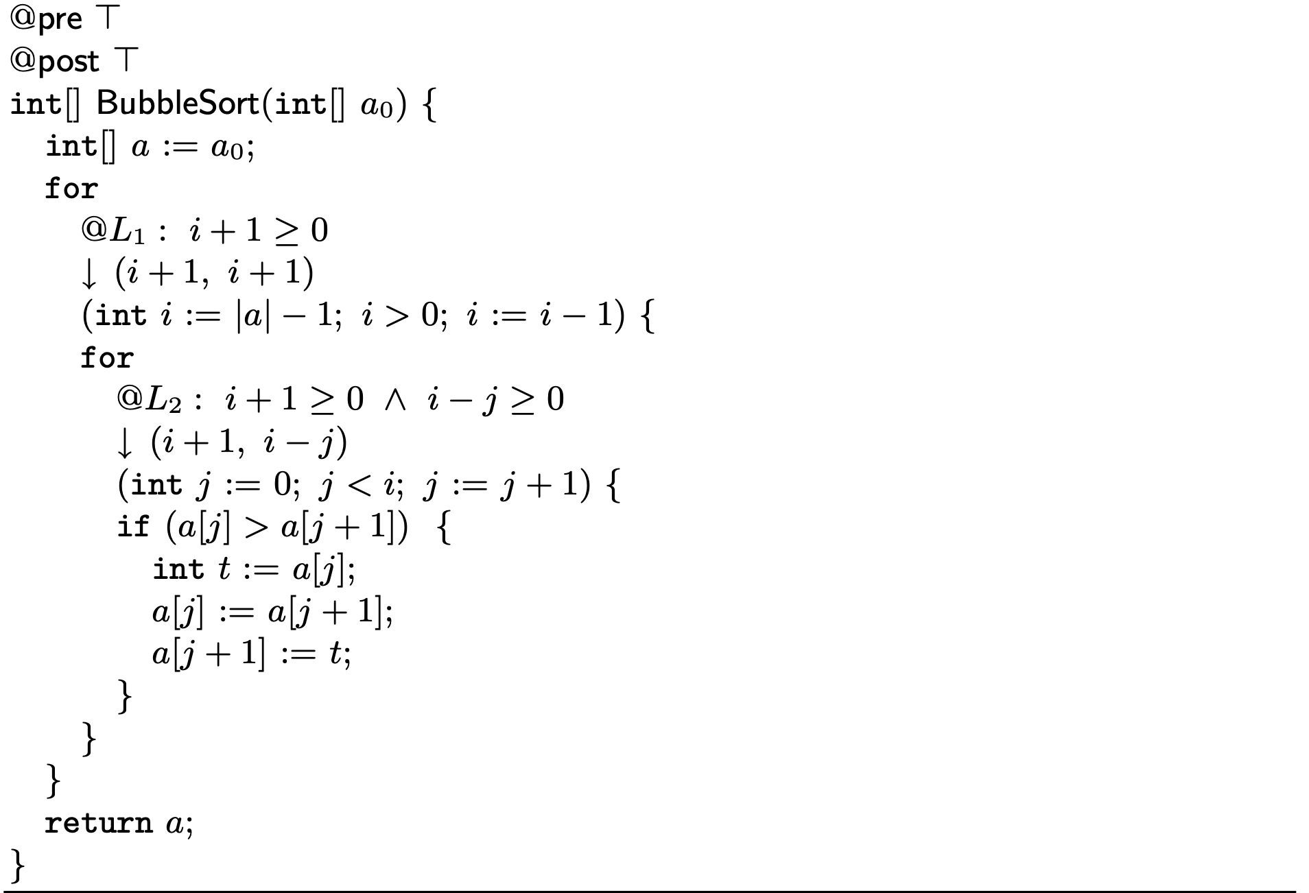
此处外层循环对应了 $\downarrow (i+1, i+1)$ ,此处使用 $i + 1$ 而不是 $i$ 的原因很简单,因为 $i := |a| - 1$,假如 $a$ 为空数组,那么长度为 0,此时计算出的 $i = -1$,由于 $i = -1$ 不是自然数,这导致无法纳入自然数元组内,进而导致无法进行后续证明,所以此处为了保证自然数属性使用了 $i + 1$ 而不是 $i$。内层循环对应的 $\downarrow (i+1, i-j)$,由于 `for` 循环内的约束,这导致不会出现 $i - j < 0$ 的情况。
在 Dafny 内,Dafny 会对每一个循环进行停机证明,大部分情况下,Dafny 可以猜到 rank function,但是在部分情况下,还是需要开发者手动指定,示例如下:
```java
method m(m: nat, n: int)
requires m <= n
{
var i := m;
while i < n
invariant 0 <= i <= n
decreases n - i
{
i := i + 1;
}
}
```
根据文档,可以使用 `decreases *` 关闭对循环的停机证明。
与前文类似,接下来,我们介绍如何手动进行证明,首先 rank functions 作为一个新的 annotation,我们可以编写一个包含 rank funcions 的 basic path,此处仅举出一个例子:
$$
\begin{array}{l}
\text{@}L_2: i+1 \ge 0\land i - j \ge 0\\
\downarrow L_2: (i+1, i - j)\\
\text{assume} \quad j \ge i;\\
i := i - 1;\\
\downarrow L_1: (i+1, i+1)\\
\end{array}
$$
上述 path 可以被抽象为:
$$
\begin{array}{l}
@ F\\
\downarrow \delta[\bar{x}]\\
S_1;\\
\vdots\\
S_k;\\
\downarrow \kappa[\bar{x}]
\end{array}
$$
可以使用如下 VC:
$$
F \to wp(\kappa \prec \delta[\bar{x}_0], S_1; \cdots; S_k)\{\bar{x}_0 \mapsto \bar{x}\}
$$
使用自然语言描述,就是为了证明在经过 $S_1, \cdots, S_k$ 语句后 $\kappa$ 的值相比于执行前的 $\delta$ 已经减少了。但是需要注意,我们在最开始 VC 推导时使用是 $\delta[\bar{x}_0]$,在最后,我们需要进行重命名操作,将命题内的 $\bar{x}_0$ 再替换为 $\bar{x}$。
我们可以将上文给出的 basic path 进行证明:
$$
\begin{align*}
\mathrm{wp}&((i+1,i+1) <_2 (i_0 + 1, i_0 - j_0), \texttt{assume }j\ge i; i:= i - 1)\\
&\iff \mathrm{wp}(\mathrm{wp}(((i-1)+1,(i-1)+1) <_2 (i_0 + 1, i_0 - j_0)), \texttt{assume }j\ge i)\\
&\iff \mathrm{wp}((i, i) <_2 (i_0 + 1, i_0 - j_0), \texttt{assume }j\ge i)\\
&\iff j \ge i \to (i, i) <_2 (i_0 + 1, i_0 - j_0)
\end{align*}
$$
然后使用 $\bar{x}_0 \mapsto \bar{x}$ 进行换元,获得 $j \ge i \to (i, i) <_2 (i + 1, i - j)$。然后增加 $F \to$ 部分,最终获得:
$$
i+1 \ge 0\land i - j \ge 0 \land j \ge i \to (i,i) <_2 (i+1, i-j)
$$
显然,因为 $i < i + 1$ ,所以上述 VC 一定是 valid 的。
## 总结
在本文中,我们从最基础的 FOL 为读者介绍最基础的逻辑学知识,然后引入了基于 theory 的 SMT 概念,这是后续证明的基石概念。至此,我们就补充了后文所需的大部分逻辑学知识。
在本文的第二大部分,我们主要讨论了程序的正确性,介绍了一系列工具辅助开发者可以对一段代码进行证明,并且介绍了使用 wp 函数将 basic path 的证明转化为对 VC 的证明。最后,我们介绍了递归方法,特别是 Well-founded induction 以及在停机证明中的使用。
正如文章开头所述,本文介绍的内容几乎约等于纸笔作业,核心的 VC 部分,我们都是手动使用 wp 函数完成的推导,但本文也给出了 dafny 的语法。在下一篇文章内,我们会使用 dafny 证明一些更加有趣的代码。有可能会介绍 [Verification of the Deposit Smart Contract in Dafny](https://github.com/Consensys/deposit-sc-dafny) 内的部分证明。
## Verification Conditions
在上一节中,我们介绍了如何获得一段代码的 path,我们可以看到每一段 path 都是存在开始状态、动作和结束状态,我们一般使用 *Hoare triple* 表示:
$$
\{F\}S_1;\dots;S_n\{G\}
$$
我们需要证明在初始状态 $F$ 的情况下,经过 $S_1; \dots; S_n$ 语句操作后,最终获得的状态为 $G$。在具体的证明过程中,我们会使用被称为 weakest precondition 的机制。
weakest precondition $\mathrm{wp}(F,S)$ ,此处的 $F$ 指的是任意 FOL 表达式,而 $S$ 指程序语句。wp 的定义为如果程序状态 s 满足 $s \models \mathrm{wp}(F, S)$ 且此处的 $S$ 语句在状态 $s$ 操作后获得的状态 $s'$ 满足 $s' \models F$。换言之,假如结束状态满足 $F$,那么其前一个状态是满足 $\mathrm{wp}(F,S)$ 的。我们可以发现 $\mathrm{wp}(F,S)$ 提供了一种方法,允许我们将对 $\{F\}S_1;\dots;S_n\{G\}$ 的 correctness 证明转化为对单一命题的证明,方法是进行进行类似如下的调用:
$$
\mathrm{wp}(\mathrm{wp}(\mathrm{wp}(\mathrm{wp}(G, S_n), S_{n-1}), \dots),F)
$$
根据 wp 的定义,假如上述 FOL 是 valid 的,那么就意味着程序在任意状态下都是正确的。假如读者无法理解上述描述,也可以继续阅读,因为实际上无法理解原理也可以使用 wp 方法证明程序的正确性。
对于 Assumption 和 Assignment 语句而言,定义 wp 为:
1. $\mathrm{wp}(F, \text{assume } c) \iff c \to F$
2. $\mathrm{wp}(F[v], v:= e) \iff F[e]$,该表达式含义是将命题 $F$ 内的变量 $v$ 替换为 $e$,命题仍成立
对于一系列语句 $S_1; \dots; S_n$ ,我们定义:
$$
\mathrm{wp}(F, S_1; \dots; S_n) \iff \mathrm{wp}(\mathrm{wp}(F, S_n), S_1; \dots, S_{n-1})
$$
简单来说,我们会按照从后到前的顺序依次使用语句 $S$ 调用 wp 函数,此处的定义与上文的分析是一致的。对任意 basic path $\{F\}S_1;\dots;S_n\{G\}$ 而言,其 verification condition 为:
$$
F \to \mathrm{wp}(G, S_1, \dots, S_n)
$$
实际上我们只需要证明上述 verification condition 的 valid 属性,就可以证明对应的 basic path 的正确性。上述 verification condition 其实与 $\mathrm{wp}(\mathrm{wp}(\mathrm{wp}(\mathrm{wp}(G, S_n), S_{n-1}), \dots),F)$ 是一致的,我们只是将最终的 $\mathrm{wp}(\dots, F)$ 利用 Assumption 语句展开为了 $F \to \mathrm{wp}(G, S_1, \dots, S_n)$。
举例说明,以下 path 来自LinearSearch 的 path (2):
$$
\begin{array}{l}
\text{@F:}\quad \ell \le i \land (\forall j. \ell \le j < i \to a[j] \ne e)\\
S_1\text{ : }\texttt{assume } i \le u;\\
S_2\text{ : }\texttt{assume } a[i] = e;\\
S_3\text{ : }rv := \texttt{true};\\
\text{@post G:}\quad rv \leftrightarrow \exists j. \ell \le j \le u \land a[j] = e
\end{array}
$$
上述代码的 VC 是 $F \to \mathrm{wp}(G, S_1; S_2; S_3)$,我们首先计算 wp 函数部分:
$$
\begin{align*}
\mathrm{wp}&(G, S_1; S_2; S_3)\\
&\iff \mathrm{wp}(\mathrm{wp}(rv \leftrightarrow \exists j. \ell \le j \le u \land a[j] = e , rv := \texttt{true}), S_1; S_2)\\
&\iff \mathrm{wp}(\texttt{true} \leftrightarrow \exists j. \ell \le j \le u \land a[j] = e, S_1;S_2)\\
&\iff \mathrm{wp}(\exists j. \ell \le j \le u \land a[j] = e, S_1;S_2)\\
&\iff \mathrm{wp}(\mathrm{wp}(\exists j. \ell \le j \le u \land a[j] = e, \texttt{assume } a[i] = e), S_1)\\
&\iff \mathrm{wp}(a[i] = e \to \exists j. \ell \le j \le u \land a[j] = e, S_1)\\
&\iff \mathrm{wp}(a[i] = e \to \exists j. \ell \le j \le u \land a[j] = e, \texttt{assume } i \le u)\\
&\iff i\le u \to (a[i] = e \to \exists j. \ell \le j \le u \land a[j] = e)
\end{align*}
$$
完整的 VC 应该是:
$$
\begin{align*}
\ell &\le i \land (\forall j. \ell \le j < i \to a[j] \ne e)\\
& \to i\le u \to (a[i] = e \to \exists j. \ell \le j \le u \land a[j] = e)
\end{align*}
$$
在本文最开始,我们证明过 $F: A \to B \to C \iff (A \land B) \to C$,该命题的泛化版本是:
$$
F_1 \to F_2 \to \dots \to F_n \iff (F_1 \land \dots \land F_{n-1}) \to F_n
$$
所以上述 VC 可以被转化为:
$$
\begin{align*}
\ell &\le i \land (\forall j. \ell \le j < i \to a[j] \ne e) \\
& \land i\le u \land a[i] = e \to (\exists j. \ell \le j \le u \land a[j] = e)
\end{align*}
$$
读者可以直接把这个命题丢给 LLM 处理,此处笔者将上述命题丢给了 ChatGPT 处理获得了如下 smt2 代码:
```lisp
(set-logic AUFLIA)
(declare-sort Elem 0)
(declare-const l Int)
(declare-const i Int)
(declare-const u Int)
(declare-const e Elem)
(declare-const a (Array Int Elem))
(define-fun F () Bool
(=> (and
(<= l i)
(forall ((j Int))
(=> (and (<= l j) (< j i))
(not (= (select a j) e))))
(<= i u)
(= (select a i) e))
(exists ((j Int))
(and (<= l j)
(<= j u)
(= (select a j) e)))))
(assert (not F))
(check-sat)
```
输出结果应该是 `unsat`,说明 VC 是 valid 的,也可以证明 LinearSearch 的部分正确性,完全的正确性需要证明所有的 path 对应的 VC 都是 valid 的。后续的文章中,我们不会处理 VC 最终的证明,读者可以直接丢给 LLM 处理为 smt2 语言,然后由 z3 或者任何其他求解器处理。
我们可以看一个稍微有一点复杂的,BinarySearch 内的 path (2):
$$
\begin{array}{l}
\text{@pre F}\quad 0 \le \ell \land u < |a| \land \text{sorted}(a, \ell, u)\\
S_1\text{ : }\texttt{assume}\quad \ell \le u;\\
S_2\text{ : }m := (\ell + u)\ \texttt{div}\ 2;\\
S_3\text{ : }\texttt{assume}\quad a[m] = e; \\
S_4\text{ : }rv := \texttt{true};\\
\text{@post G}\quad rv \iff \exists i. \ell \le i \le u \land a[i] = e
\end{array}
$$
还是首先计算 $\mathrm{wp}(G, S_1; S_2; S_3; S_4)$ 部分:
$$
\begin{align*}
\mathrm{wp}&(G, S_1; S_2; S_3; S_4)\\
&\iff \mathrm{wp}(\mathrm{wp}(G, S_4), S_1; S_2; S_3)\\
&\iff \mathrm{wp}(\mathrm{wp}(G, rv := \texttt{true}), S_1; S_2; S_3)\\
&\iff \mathrm{wp}(\mathrm{wp}(G\{rv \mapsto \texttt{true}\}), S_1; S_2; S_3)\\
&\iff \mathrm{wp}(\mathrm{wp}(G\{rv \mapsto \texttt{true}\}, S_3), S_1; S_2)\\
&\iff \mathrm{wp}(\mathrm{wp}(G\{rv \mapsto \texttt{true}\}, \texttt{assume }a[m] = e), S_1; S_2)\\
&\iff \mathrm{wp}(a[m] = e \to G\{rv \mapsto \texttt{true}\}, S_1; S_2)\\
&\iff \mathrm{wp}(\mathrm{wp}(a[m] = e \to G\{rv \mapsto \texttt{true}\}, S_2), S_1)\\
&\iff \mathrm{wp}(\mathrm{wp}(a[m] = e \to G\{rv \mapsto \texttt{true}\}, m := (\ell + u)\ \texttt{div}\ 2), S_1)\\
&\iff \mathrm{wp}((a[m] = e \to G\{rv \mapsto \texttt{true}\})\{m \mapsto (\ell + u)\ \texttt{div}\ 2\}, S_1)\\
&\iff \mathrm{wp}((a[m] = e \to G\{rv \mapsto \texttt{true}\})\{m \mapsto (\ell + u)\ \texttt{div}\ 2\}, \texttt{assume } \ell \le u)\\
&\iff \ell \le u \to (a[m] = e \to G\{rv \mapsto \texttt{true}\})\{m \mapsto (\ell + u)\ \texttt{div}\ 2\}\\
&\iff \ell \le u \to (a[m] = e) \{m \mapsto (\ell + u)\ \texttt{div}\ 2\} \to G\{rv \mapsto \texttt{true}, m \mapsto (\ell + u)\ \texttt{div}\ 2\}\\
&\iff \ell \le u \to a[(\ell + u)\ \texttt{div}\ 2] = e \to G\{rv \mapsto \texttt{true}, m \mapsto (\ell + u)\ \texttt{div}\ 2\}\\
&\iff \ell \le u \to a[(\ell + u)\ \texttt{div}\ 2] = e \to \exists i. \ell \le i \le u \land a[i] = e
\end{align*}
$$
上述化简的最后 3 步都是在处理赋值问题,其实只需要将变量名对应的值带入 FOL 即可,假如该变量名不存在,比如 $G$ 中不存在 $m$ 变量,那么就可以忽略。
BubbleSort 的 path (3) 是一个相当复杂的案例,我们在此处只给出最终的结果:

## Total Correctness
在上一节中,我们介绍了如何使用基于 wp 的 VC 机制证明程序的 Partial correctness 属性,利用上述方法可以证明程序的 basic path 正确性,更加严谨来说,上述方法可以证明程序的任意状态都是符合我们预期的,但是上述方法无法证明程序会停机。在本节中,我们主要提供一种使用 ranking function 的方法。
在介绍具体的方法前,我们需要补充一个背景知识,即 *well-founded relation*。假设在集合 $S$ 上存在一个 binary predicate $\prec$ ,我们称 $\prec$ 是 well-founded relation 在有且仅有 $S$ 集合 **不存在** 无限长的序列 $s_1, s_2, \dots$ 满足 successive element 小于 predecessor:
$$
s_1 \succ s_2 \succ s_3 \succ \dots
$$
并且上述关系中存在 $s \succ t \iff t \prec s$。换言之,well-founded relation 要求集合 $S$ 内对 $\prec$ 关系只存在有限长度的序列。我们举例说明,对于自然数上的 $<$ 而言,$<$ 关系是满足 well-founded relation,因为任意的自然数序列在递减到 0 后就停止了,所以不存在基于 $<$ 构造的无限长度序列。但是在有理数集合内,$<$ 关系不是 well-founded relation,因为有理数集合可以出现以下递减序列:
$$
1 > \frac{1}{2} > \frac{1}{3} > \frac{1}{4} > \dots
$$
我们可以在有理数集合内可以构造出无限长的递减序列,所以有理数内的 $<$ 不是 well-founded relation。基于 well-founded relation,我们会用到一个派生概念 lexicographic relations。假设存在多个具有 well-founded relation 定义的集合的 $(S_1, \prec_1), (S_2, \prec_2), \dots, (S_m, \prec_m)$,基于此我们构建一个大的集合:
$$
S = S_1 \times \dots \times S_m
$$
对于 $s_i, t_i \in S_i$ ,定义以下 relation $\prec$
$$
(s_1, \ldots, s_m) \prec (t_1, \ldots, t_m)
\iff
\bigvee_{i=1}^{m}
\left(
s_i \prec_i t_i
\,\land\,
\bigwedge_{j=1}^{i-1} s_j = t_j
\right)
$$
上述 relation 的本质是对于元组 $s, t$ 内的元素进行逐一比较,直到找到第一个存在 $\prec$ 关系的元素,比如假设 $s = (3, 9, 10)$ 而 $t = (3, 11, 0)$,我们首先比较发现 $s_1 = t_1$,然后比较 $s_2 < t_2$,此时发现第一个满足 $\prec$ 的元素,那么 $s \prec t$ 是成立的,注意我们不关心 $s_3, t_3$ 的大小关系。对于这种自然数元组的 lexicographic 关系,我们通常使用 $<_n$ 表示,其中 $n$ 代表比较元组的长度,比如刚刚的示例其实就是 $<_3$
很多读者可能知道数学归纳法,对于自然数 $x$ 内的命题 $F[x]$ 标准的数学归纳法为:
1. base case: 证明 $F[0]$ 是 valid 的
2. inductive step: **假设**对于任意自然数 $n$,$F[n]$ 是 valid 的(即 inductive hypothesis,或缩写为 IH),我们需要证明 $F[n + 1]$ 也是 valid
当我们完成上述步骤后,我们就可以证明 $F[x]$ 对所有的自然数 $x$ 都是 valid 的。数学归纳法成立的原因是在自然数 $T_{\mathrm{PA}}$ 内存在以下公理(这个公理在本文开始介绍 theory 时也有出现):
$$
F[0] \land (\forall n. F[n] \to F[n+1]) \to \forall x. F[x]
$$
与之等价的还有另一种更加紧凑的表达递归过程公理的命题模版,如下:
$$
(\forall n. (\forall n'. n' < n \to F[n']) \to F[n]) \to \forall x. F[x]
$$
首先,此处的 inductive hypothesis 是对于任意自然数 $n$,已知 $n' < n$ 下,$F[n']$ 是 valid 的,我们需要在上述假设(即 $\forall n'. n' < n \to F[n']$) 基础上,证明 $F[n]$ 也是 valid。由于上述公理的存在,那么 $\forall x. F[x]$ 自然也是 valid 的。
上述命题实际上只表示了递归中的 inductive step 而没有包含 base case。但在很多情况下,base case 是隐含的,但有时候需要单独证明 $F[0]$ 的 valid 属性。比如在自然数情况下,不存在 $n' < 0$ 的情况,这说明 inductive step 没有隐含 base case ,所以需要单独证明 $F[0]$ 的 valid 属性。
举例说明,我们在自然数内引入如下两条与余数(remainder)有关的定理:
$$
\begin{array}{l}
\forall x,y. x < y \to rem(x,y) = x\\
\forall x, y. y > 0 \to rem(x + y, y) = rem(x, y)
\end{array}
$$
举一个具体数值计算 $rem(5, 3) = 2$。我们希望证明 $\forall y > 0 \to rem(x, y) < y$,即余数(remainder)总是小于除数(divisor)。
首先,我们可以直接给出 inductive hypothesis,此处我们选择对 $x$ 进行归纳,即对于任意的 $x$ 都存在(以下将 $n$ 替换为 $x$ 以及将 $n'$ 替换为 $x'$ 的操作是有一定危险的,因为 FOL 内存在量词约束变量,具体的安全替换方法可以参考参考书的 **2.4.1 Safe Substitution**)
$$
\forall y. y > 0 \to \forall x.((\forall x'. x' < x \to rem(x', y) < y) \to rem(x, y) < y)
$$
假如我们可以证明 $\forall x.((\forall x'. x' < x \to rem(x', y) < y) \to rem(x, y) < y)$ 是 valid 的,那么就可以证明 $\forall y. y > 0 \to \forall x. rem(x, y) < y$,这与我们希望证明的命题其实是等价的。对于形如 $H \to G$ 的待证明的命题,最简单的使用 $H$ 作为已知条件,对 $G$ 进行约化。
当然,此处存在两种情况 $x < y$ 以及 $\neg(x < y)$。对于 $x < y$ 的情况,我们有:
$$
rem(x, y) = x < y
$$
调用 $\forall x,y. x < y \to rem(x,y) = x$ 公理不难获得上述结论。对于 $\neg(x < y)$ 的情况,我们取 $x' = x - y$可以获得:
$$
rem(x, y) = rem(x', y) < y
$$
此处 $rem(x', y) < y$ 来自 inductive hypothesis。至此,我们证明了命题的 valid,也意味着最初的 $\forall y > 0 \to rem(x, y) < y$ 是 valid 的。
此处我们将本节最初介绍的 well-founded relation 引入,实际上 well-founded relation 和派生的 lexicographic relations 也可以进行归纳,这种归纳方法被称为 Well-founded induction,可以使用如下模版表示:
$$
(\forall n. (\forall n'. n' \prec n \to F[n']) \to F[n]) \to \forall x. F[x]
$$
我们在此处举一个有趣的例子。假设我们手中有一个袋子,袋子内装有 red / yellow / blue 三种颜色的小球,假如袋子内只剩一个小球,我们将其拿出来。但在其他情况下,我们随机拿走 2 个小球:
1. 假如拿走的小球其中一个是 red,我们不需要向袋子内放入小球
2. 假如拿走的两个小球都是 yellow,此时我们向袋子内放入 1 个 yellow 球和 5 个 blue 球
3. 假如其中一个是 blue 而另一个 **不是** red 球,那么向袋子放入 10 个 red 球
上述三个情况可以覆盖所有的 2 个球的可能性。问题是上述拿球的过程是否会终止?
我们首先定义一个代表袋子中三种颜色球的数目的元组 $(\# \text{yellow}, \# \text{blue}, \# \text{red})$ ,并在此基础上定义 $<_3$ lexicographic。我们需要证明无论 $(y, b, r)$ 元组内的数值最初是多少,最终通过有限的步骤变成 $(0, 0, 0)$。此处我们使用递归方法。
对于 base case 而言,我们考虑第一种 base case 就是 $(0, 0, 0)$,此时袋子中没有任何球,游戏结束。另一种可能性是袋子内只存在 1 个球,比如 $(1, 0, 0), (0, 1, 0),(0, 0, 1)$,此时只需要在进行一轮游戏拿走这一个仅剩的球就可以结束游戏。
我们的 inductive hypothesis 是对于 $(y', b', r') <_3 (y, b, r)$ 的状态,在有限步骤后游戏会结束。可以考虑一下三种情况:
1. 拿走红球后,袋子状态为 $(y - 1, b, r - 1), (y, b-1, r-1), (y, b, r-2)$,分别对应三种不同情况,我们可以发现每种情况都满足 $<_3 (y, b, r)$,基于 inductive hypothesis,有限步骤后游戏结束
2. 拿走的两个小球都是 yellow,袋子状态为 $(y - 1, b + 5, r)$ 也满足 $<_3 (y, b, r)$ 的情况,基于 inductive hypothesis,有限步骤后游戏结束
3. 拿走的小球其中一个是 blue 而另一个不是 red,袋子状态可能是 $(y - 1, b - 1, r+10), (y, b - 2, r + 10)$ 两种可能状态都满足 $<_3$ 所以基于 inductive hypothesis,有限步骤后游戏结束
至此,我们就使用 lexicographic 证明了系统会在有限步骤内停止。这也是本节最初介绍程序停机证明的原理。而一直提到的 ranking function 会将程序状态映射到一个满足 well-founded relation $\prec$ 的集合 $S$ 内。我们一般会使用上文介绍的定义在自然数元组上的 $<_n$ 作为集合 $S$ 的 well-founded relation 。在实际工程中,我们往往使用是一种特殊的 annotations 代表 rank function。如下图所示代码内的 $\downarrow (i+1, i+1)$ 和 $\downarrow (i+1, i-j)$ 都是 rank function:

此处外层循环对应了 $\downarrow (i+1, i+1)$ ,此处使用 $i + 1$ 而不是 $i$ 的原因很简单,因为 $i := |a| - 1$,假如 $a$ 为空数组,那么长度为 0,此时计算出的 $i = -1$,由于 $i = -1$ 不是自然数,这导致无法纳入自然数元组内,进而导致无法进行后续证明,所以此处为了保证自然数属性使用了 $i + 1$ 而不是 $i$。内层循环对应的 $\downarrow (i+1, i-j)$,由于 `for` 循环内的约束,这导致不会出现 $i - j < 0$ 的情况。
在 Dafny 内,Dafny 会对每一个循环进行停机证明,大部分情况下,Dafny 可以猜到 rank function,但是在部分情况下,还是需要开发者手动指定,示例如下:
```java
method m(m: nat, n: int)
requires m <= n
{
var i := m;
while i < n
invariant 0 <= i <= n
decreases n - i
{
i := i + 1;
}
}
```
根据文档,可以使用 `decreases *` 关闭对循环的停机证明。
与前文类似,接下来,我们介绍如何手动进行证明,首先 rank functions 作为一个新的 annotation,我们可以编写一个包含 rank funcions 的 basic path,此处仅举出一个例子:
$$
\begin{array}{l}
\text{@}L_2: i+1 \ge 0\land i - j \ge 0\\
\downarrow L_2: (i+1, i - j)\\
\text{assume} \quad j \ge i;\\
i := i - 1;\\
\downarrow L_1: (i+1, i+1)\\
\end{array}
$$
上述 path 可以被抽象为:
$$
\begin{array}{l}
@ F\\
\downarrow \delta[\bar{x}]\\
S_1;\\
\vdots\\
S_k;\\
\downarrow \kappa[\bar{x}]
\end{array}
$$
可以使用如下 VC:
$$
F \to wp(\kappa \prec \delta[\bar{x}_0], S_1; \cdots; S_k)\{\bar{x}_0 \mapsto \bar{x}\}
$$
使用自然语言描述,就是为了证明在经过 $S_1, \cdots, S_k$ 语句后 $\kappa$ 的值相比于执行前的 $\delta$ 已经减少了。但是需要注意,我们在最开始 VC 推导时使用是 $\delta[\bar{x}_0]$,在最后,我们需要进行重命名操作,将命题内的 $\bar{x}_0$ 再替换为 $\bar{x}$。
我们可以将上文给出的 basic path 进行证明:
$$
\begin{align*}
\mathrm{wp}&((i+1,i+1) <_2 (i_0 + 1, i_0 - j_0), \texttt{assume }j\ge i; i:= i - 1)\\
&\iff \mathrm{wp}(\mathrm{wp}(((i-1)+1,(i-1)+1) <_2 (i_0 + 1, i_0 - j_0)), \texttt{assume }j\ge i)\\
&\iff \mathrm{wp}((i, i) <_2 (i_0 + 1, i_0 - j_0), \texttt{assume }j\ge i)\\
&\iff j \ge i \to (i, i) <_2 (i_0 + 1, i_0 - j_0)
\end{align*}
$$
然后使用 $\bar{x}_0 \mapsto \bar{x}$ 进行换元,获得 $j \ge i \to (i, i) <_2 (i + 1, i - j)$。然后增加 $F \to$ 部分,最终获得:
$$
i+1 \ge 0\land i - j \ge 0 \land j \ge i \to (i,i) <_2 (i+1, i-j)
$$
显然,因为 $i < i + 1$ ,所以上述 VC 一定是 valid 的。
## 总结
在本文中,我们从最基础的 FOL 为读者介绍最基础的逻辑学知识,然后引入了基于 theory 的 SMT 概念,这是后续证明的基石概念。至此,我们就补充了后文所需的大部分逻辑学知识。
在本文的第二大部分,我们主要讨论了程序的正确性,介绍了一系列工具辅助开发者可以对一段代码进行证明,并且介绍了使用 wp 函数将 basic path 的证明转化为对 VC 的证明。最后,我们介绍了递归方法,特别是 Well-founded induction 以及在停机证明中的使用。
正如文章开头所述,本文介绍的内容几乎约等于纸笔作业,核心的 VC 部分,我们都是手动使用 wp 函数完成的推导,但本文也给出了 dafny 的语法。在下一篇文章内,我们会使用 dafny 证明一些更加有趣的代码。有可能会介绍 [Verification of the Deposit Smart Contract in Dafny](https://github.com/Consensys/deposit-sc-dafny) 内的部分证明。