---
title: Demo_11
tags: MF
---
# Fraudulent Firms Detection via Binary Classification in Audit Risk Scores
#### keywords: *fraud detection*, *binary classification*, *audit risk*, *logistic regression*, *random forest*, *SVM*, *KNN*, *neural network*
:::info
陽交大資財系機器學習與金融科技期末報告,由許智超,李亦涵,鄧惠文共同編輯。最後更新時間2021/11/22。
:::
---
## 1. Motivations
I am interested in building a ***classification model*** in detecting ***fraudulent firms***, to help auditors reduce the ***audit risk***.

---
## 2. Data Visualization (EDA)
有關各領域(sectors)的公司數量:
||||
|:---:|:---:|:---:|
|灌溉Irrigation (114)|公共衛生Public Health (77)|建築與道路Buildings and Roads (82)|
|森林Forest (70)|一般企業Corporate (47)|畜牧業Animal Husbandry (95)|
|傳播Communication (1)|電子Electrical (4)|土地Land (5)|
|科學科技業Science and Technology (3)|旅遊業Tourism (1)|漁業Fisheries (41)|
|工業Industries (37)|農業Agriculture (200)|
---
### 名詞解釋
- **財報審計**:
1. 財報是否有恰當地編制?
2. 公允反應財務信息?
- **審計風險(audit risk)**: 審計師發表不恰當的審計意見的風險
$$審計風險(audit\ risk) = $$
$$=重大錯報風險(material\ misstatement\ risk) \times 檢查風險(detection\ risk)$$
$$= (固有風險(inherent\ risk) \times 控制風險(control\ risk)) \times 檢查風險(detection\ risk)$$
---
- **重大錯報風險(material misstatement risk)**:
1. 與審計師無關
2. 固有風險 $\times$ 控制風險
- **固有風險(inherent risk)**:
> 例如:會計人員將200元記錄成200萬元的風險。
- **控制風險(control risk)**:
> 例如:會計人員將200元記錄成200萬元了,而會計主管也未能即時發現並糾正的風險。
- **檢查風險(detection risk)**:
1. 只與審計師相關
2. 不可能將發生率降至0
> 例如: 會計人員將200元記錄成200萬元了,而會計主管也未能即時發現並糾正,然後審計人員測試時還是沒有發現的風險。
**條件機率!?**
---
### 變數說明
### 固有風險因子(Inherent Risk Factors)
|Variables|Columns|Descriptions|
|---|---|---|
|$x_A$|**PARA_A**|稽核(inspection)中的*計畫支出(planned expenditure)* 總額,與財報A(summary report A)之間,分歧(discrepancy)的總金額,單位是印度貨幣「盧比Rs」。我們代稱此為「A情況」|
|$p_A$|**Score_A**|上述分歧發生的機率值,此稱「分數A」|
|$risk_A$|**Risk_A**|風險分數A = A情況損失總額 $\times$ 機率值 = "PARA_A" $\times$ "Score_A"|
---
|Variables|Columns|Descriptions|
|---|---|---|
|$x_B$|**PARA_B**|稽核(inspection)中的*非計畫支出(unplanned expenditure)* 總額,與財報B(summary report B)之間,分歧(discrepancy)的總金額,單位是印度貨幣「盧比Rs」。我們代稱此為「B情況」|
|$p_B$|**Score_B**|上述分歧發生的機率值,此稱「分數B」|
|$risk_B$|**Risk_B**|風險分數B = B情況損失總額 $\times$ 機率值 = "PARA_B" $\times$ "Score_B"|
|<hr/>|<hr/>|
|$total_{AB}$|**TOTAL**|上述兩種分歧情況加總的總損失金額,也就是"PARA_A" $+$ "PARA_B"|
---
|Variables|Columns|Descriptions|
|---|---|---|
|$x_c$|**numbers**|歷史資料的分歧分數(historical discrepancy score)|
|$p_c$|**Risk_B.1**|對應上述歷史資料分歧分數,類似機率值/權重的東西|
|$risk_C$|**Risk_C**|風險分數C = 歷史分歧分數 $\times$ 對應權重 = "numbers" $\times$ "Risk_B.1"|
---
|Variables|Columns|Descriptions|
|---|---|---|
|$x_D$|**Money_Value**|過去的審計中,錯報(misstatements)的金額總額|
|$p_D$|**Score_MV**|對應上述歷史錯報金額總額,類似機率值/權重的東西|
|$risk_D$|**Risk_D**|風險分數D = 歷史錯報金額總額 $\times$ 對應權重 = "Money_Value" $\times$ "Score_MV"|
|<hr/>|<hr/>|
|$total_{in}$|**Inherent_Risk**|就是總固有風險分數|
---
### 控制風險因子(Control Risk Factors)
|Variables|Columns|Descriptions|
|---|---|---|
|$x_{SS}$|**Sector_score**|根據每筆資料所屬的部門(sector),使用一些分析程序計算出來的,該部門的歷史風險分數(historical risk score)|
---
|Variables|Columns|Descriptions|
|---|---|---|
|$x_E$|**District_Loss**|一個區域(district)在*近10年內(in the last 10 years)* 的歷史風險分數(historical risk score)
|$p_E$|**PROB**|對應上述某區域10年內歷史風險分數,類似機率值/權重的東西|
|$risk_E$|**RiSk_E**|風險分數E = 某區域10年內歷史風險分數 $\times$ 對應權重 = "District_Loss" $\times$ "PROB"|
---
|Variables|Columns|Descriptions|
|---|---|---|
|$x_F$|**History**|此公司*近10年內*的歷史損失(historical loss)的平均(average)|
|$p_F$|**Prob**|對應上述公司10年內的歷史損失平均,類似機率值/權重的東西|
|$risk_F$|**Risk_F**|風險分數F = 公司10年內的歷史損失平均 $\times$ 對應權重 = "History" $\times$ "Prob"|
|<hr/>|<hr/>|
|$total_{co}$|**CONTROL_RISK**|就是總控制風險分數|
---
### 檢查風險因子(Detection Risk Factors)
|Variables|Columns|Descriptions|
|---|---|---|
|$risk_{DR}$|**Detection_Risk**|就是檢查風險分數|
---
### 其他特徵(Other Features)
|Variables|Columns|Descriptions|
|---|---|---|
|$x_{loc}$|**LOCATION_ID**|每筆資料所屬城市/省份的唯一ID編號|
|$x_s$|**Score**|不明分數,資料來源論文並未敘明|
---
|Variables|Columns|Descriptions|
|---|---|---|
|$y_{score}$|**Audit_Risk**|使用一些分析程序計算出來的總風險分數(total risk score)|
|$y$|**Risk**|每筆資料是否為詐欺公司的二元類別變數。***This is the target feature!***|
---
### EDA部份
```python=
#匯入函式庫
import numpy as np
import pandas as pd
import matplotlib.pyplot as plt
#這一行魔法函式可以省略每次的plt.show(),直接顯示
%matplotlib inline
import seaborn as sns
import os
#因為我們沒有testing data,所以要切一份出來
#以下EDA將會進行於trainig data
from sklearn import model_selection
#圖片樣式美化
plt.style.use('dark_background')
```
```python=
#切換工作目錄
os.chdir("C:\\Users\\GL75\\OneDrive\\桌面\\機器學習與金融科技\\Project")
#讀入資料
data = pd.read_csv('audit_data.csv')
```
```python=
#觀察資料格式
#顯示所有的行,為了觀察各變數名稱,以及它們之間的關係
pd.options.display.max_columns = None
data.head() #展示頭5筆的資料
```
---
資料的樣子


---
```python=
#列出所有行的標題,也就是變數名稱
data.columns
```

---
### 資料前處理
重新命名
```python=
#有些變數名稱不太統一,我們稍微修正,統一大小寫格式
data.rename(columns = {'RiSk_E':'Risk_E', 'LOCATION_ID':'Location_ID', 'PARA_A': 'Para_A', 'PARA_B':'Para_B', 'TOTAL': 'Total', 'PROB': 'ProbA', 'Prob': 'ProbB', 'CONTROL_RISK': 'Control_Risk'}, inplace = True)
```
<br>刪除變數Total
```python=
#因為變數TOTAL其實就等於PARA_A+PARA_B,沒有額外貢獻資訊
#因此我們drop掉這個變數
data.drop(['Total'], axis = 1, inplace = True) #inplace = True可以直接就地修改
```
---
沒有缺失值
```python=
data.info()
#可以看到總共有776筆資料,全部變數都沒有缺失值(null value)
#除了"District_Loss", "History"以及目標變數"Risk"是整數型別(int32),"LOCATION_ID"是某種object以外
#其他所有變數都是浮點數型別(float64)
```

---
敘述統計量
```python=
#以下列出基本的敘述統計量(descriptive statistics)
data.describe()
```


---
刪除變數"Detection_Risk":
1. mean = Q1 = Q3 = 0.5
2. standard deviation = 0
全是0.5?!by nunique() ... indeed!
```python=
data['Detection_Risk'].nunique()
```

```python=
data.drop(['Detection_Risk'], axis = 1, inplace = True)
```
---
刪除變數"Location_ID":
1. Unknown Data type
2. Not helpful
```python=
data['Location_ID'].dtypes
```

```python=
data.drop(['Location_ID'], axis = 1, inplace = True)
```
---
相關係數
```python=
#首先是熱力圖heatmap
plt.figure(figsize = (20, 20))
sns.heatmap(data.corr(), annot = True, cmap = 'coolwarm')
plt.savefig("heatmap.png")
```

---
1. "Sector_score"跟其他變數之間都呈現負相關。
> 特別是"Score_A", "Score_MV", "Score" 和 "Risk"。
2. 有些變數間有極高的正相關:
* **完全正相關(1或0.99)**:
||||||
|:---:|:---:|:---:|:---:|:---:|
|Para_A|Para_B|Score_B.1|Money_Value|Risk_F|
|Risk_A|Risk_B|Risk_C|Risk_D|History|
* **極高度正相關(0.9以上)**:
|||||||
|:---:|:---:|:---:|:---:|:---:|:---:|
|numbers|numbers|District_Loss|Score_B|Audit_Risk|Audit_Risk|
|Score_B.1|Risk_C|Risk_E|Score|Para_B|Risk_B|
保留變數:
> **完全正相關**: "Risk_A"、"Risk_B"、"Risk_C"、"Risk_D" 和 "Risk_F"
> **極高度正相關**: "Score_B.1", "Risk_E"。
至於變數"Score"因為我們不了解,因此不會隨意刪除。
故"Score"與"Score_B"這組2個都保留。
3. 刪除變數"Audit_Risk":
A. 受所有risk分數影響
B. 目標變數(target variable)"Risk"的判斷基準
```python=
data.drop(["Para_A","Para_B","Score_B.1","Money_Value","History","numbers","District_Loss","Audit_Risk"], axis = 1, inplace = True)
```
---
刪除變數後的correlation heatmap
-> better!
```python=
plt.figure(figsize = (20, 20))
sns.heatmap(data.corr(), annot = True, cmap = 'coolwarm')
plt.savefig("heatmap_deleteHighCorr.png")
```

扣除相關係數後,其他變數之間,彼此已經沒有嚴重的高相關性了。
---
相關性:目標變數 **"Risk"** vs. 其他
```python=
#首先,將Risk這個變數獨立出來,叫做y,之後要當target用的,所以不要混在一起
y = data.Risk
#除此之外的其他資料就是我們要用來分類的變數dataset,叫做x
x = data.drop(['Risk'], axis = 1)
x.corrwith(y).plot.bar(figsize = (20, 10), fontsize = 20, grid = True, color = ['r','g','b'] * 3).set_title("Correlation between 'Risk' and other variables", fontsize = 20)
plt.savefig("risk_corr_with_others.png")
```

如前所述,除了變數**Sector_score**和所有其他變數之間都呈現*負相關*以外,其他變數都和目標變數**Risk**之間都呈現或多或少的正相關(相關係數從0.2~0.8左右)。
---
```python=
y = pd.DataFrame({'Risk':data['Risk']}) #把y從pandas的Series轉成DataFrame
#以便後續分析使用
```
---
樣本中的**違約比例**
```python=
sns.countplot(y['Risk'], label = 'Count')
```

```python=
y.value_counts(normalize = True)
```

> About **39.3%**
---
## 3. Problem formulation and our methods
$$
Audit\ Risk=f(Inherent\ Risk, Control\ Risk, Detection\ Risk)\\
= f(\sum_{i=A}^Drisk_i+\sum_{j=E}^Frisk_j+risk_{DR})=f(total\ risk \ score)=f(y_{score})\\
\begin{cases}
1 & \text{if total risk score} \ge {1}\\
0 & \text{if total risk score < 1}
\end{cases}\\
$$
$$
\text{Prediction = 1 denotes that the firm might be fraudulent, 0 otherwise.}
$$
我們想要找出模型$f()$,這個模型使用**審計風險**中的各種風險分數當成輸入,輸出一個二元預測值,代表這筆觀察值的公司**是否有詐欺風險存在**。
越準確越好,使用**混淆矩陣**,以及其他有關方法測量(準確率、精確率、召回率、F1分數、ROC以及AUC等等)。
**Benchmark Method**: 伯努力試驗(*Bernoulli trials*) $n$ 次。
1. 0/1分別代表可能不是/是詐欺公司。
2. $n$ = 訓練/測試資料集長度
3. $p$ = 樣本中的詐欺公司比例 $\approx$ **39.3%**
<br>**Models Used**:
1. 羅吉斯回歸(Logistic Regression)
2. 隨機森林(Random Forest) :trophy:
3. K-近鄰演算法(K Nearest Neighbor)
4. 支持向量機(Support Vector Machine)
5. 簡單神經網路(Vanilla Neural Network)
<br>**In-sample and Out-of-sample Analysis**:
```python=
from sklearn.model_selection import train_test_split
```
1. 訓練資料:驗證資料 = 3:1
2. 用ground truth的比例去做**分層抽樣 (stratified sampling)**
3. 隨機打亂資料 (*seed = 42*)
```python=
x_train, x_test, y_train, y_test = train_test_split(x, y, test_size = 0.25, stratify = y, random_state = 42)
```
---
## 4. Analysis and Conclusion
### 切割驗證資料集
請見3. problem formulation中的**In-sample and Out-of-sample Analysis**
### 資料前處理 (Data Preprocessing)
使用*sklearn*的**StandardScaler**將所有變數**標準化**
> 都是連續型
```python=
from sklearn.preprocessing import StandardScaler
```
```python=
stdScaler = StandardScaler()
#我們先用fit_transform()找出訓練資料的統計量值特徵,再用這些將訓練資料標準化
x_train_scaled = pd.DataFrame(stdScaler.fit_transform(x_train))
#然後再對測試資料直接用transform(),拿訓練資料的這些統計量值,對測試資料標準化。
#原因是我們假設他們出自相同分布,所以當然沒必要重新fit一次
x_test_scaled = pd.DataFrame(stdScaler.transform(x_test))
#要注意fit_transform()和transform不能倒過來用,不然會報錯!
```
<br>將訓練資料以及驗證資料的ground truth都轉成**ndarray**格式
```python=
y_train_np = y_train['Risk'].to_numpy()
ground_truth = y_test['Risk'].to_numpy()
```
---
### Benchmark Method: Binomial Sampling
> $n$ = 訓練/測試資料集長度
> $p$ = 39.3%
```python=
np.random.seed(42)
n_train = len(x_train_scaled.index) #縮放後訓練資料集的長度
n_test = len(x_test_scaled.index) #縮放後測試資料集的長度
p = y.value_counts(normalize = True)[1] #樣本中的有審計風險的公司比例約為39.3%,以此做為估計量
#從進行n次的白努力試驗(Bernoulli's Trials),機率約為39.3%,n取決於資料集長度
benchmark_train = np.random.binomial(1, p, n_train)
benchmark_test = np.random.binomial(1, p, n_test)
```
---
### Cross Validation for Benchmark Method
之後所有方法都用**K-fold validation**,$K=10$
```python=
Kfold = model_selection.KFold(n_splits = 10, random_state = 42, shuffle = True)
acc = []
for _, test_idx in Kfold.split(x_train_scaled):
predicted = benchmark_train[test_idx]
ground_truth = y_train['Risk'].to_numpy()[test_idx]
#計算這次fold的驗證資料的準確率(accuracy)
acc.append((predicted == ground_truth).sum() / len(test_idx))
```
<br>驗證資料的準確率(accuracy)約為
> 50.7%
```python=
acc_val = sum(acc) / len(acc)
print(acc_val)
```
<br>
---
### Model Evaluation for Benchmark Method
先求出真實答案&預測結果
```python=
ground_truth = y_test['Risk'].to_numpy()
predicted = benchmark_test
```
<br>使用*sklearn*套件中,*metrics*包裡面的**accuracy_score, f1_score, precision_score, recall_score, roc_auc_score**等方法
計算**準確率、F1分數、精確率、召回率、ROC的AUC**
```python=
from sklearn.metrics import accuracy_score, f1_score, precision_score, recall_score, roc_auc_score
```
<br>一樣,往後其他模型也都這樣做。
```python=
accuracy = accuracy_score(ground_truth, predicted)
precision = precision_score(ground_truth, predicted)
recall = recall_score(ground_truth, predicted)
F1 = f1_score(ground_truth, predicted)
ROC = roc_auc_score(ground_truth, predicted)
results_benchmark = pd.DataFrame([['Benchmark Method', accuracy, acc_val, precision, recall, F1, ROC]], columns = ['Model', 'Accuracy','Cross Val Accuracy', 'Precision', 'Recall', 'F1 Score','ROC'])
results_benchmark
```
<br>
---
### Logistic Regression
1. 加上L1懲罰項做正則化
> 減弱羅吉斯回歸模型的精度,提高泛化效果,避免過擬合(overfitting)
2. 隨機打亂數據
> *seed = 42* 方便比較
```python=
from sklearn.linear_model import LogisticRegression
logReg = LogisticRegression(random_state = 42, penalty = 'l1', solver='liblinear') #l1 penalty
logReg.fit(x_train_scaled, y_train_np)
```
---
### Cross Validation for Logistic Regression
往後方法都透過*sklearn*套件中,*model_selection*包裡面的現成函數
**cross_val_score**來進行**交叉驗證**
```python=
from sklearn.model_selection import cross_val_score
```
<br>**10-fold validation**
```python=
Kfold = model_selection.KFold(n_splits = 10, random_state = 42, shuffle = True)
scoring = 'accuracy' #我們要看交叉驗證的準確率如何
```
<br>驗證資料的準確率(accuracy)約為
> 96.4%
```python=
acc_logReg = cross_val_score(estimator = logReg, X = x_train_scaled, y = y_train_np, cv = Kfold, scoring = scoring)
acc_val = acc_logReg.mean()
print(acc_val)
```
<br>
---
### Model Evaluation for Logistic Regression
先求出真實答案&預測結果
```python=
ground_truth = y_test['Risk'].to_numpy()
predicted = logReg.predict(x_test_scaled)
```
<br>使用*sklearn*的現成函數計算performances
```python=
accuracy = accuracy_score(ground_truth, predicted)
precision = precision_score(ground_truth, predicted)
recall = recall_score(ground_truth, predicted)
F1 = f1_score(ground_truth, predicted)
ROC = roc_auc_score(ground_truth, predicted)
results_logReg = pd.DataFrame([['Logistic Regression', accuracy, acc_val, precision, recall, F1, ROC]], columns = ['Model', 'Accuracy','Cross Val Accuracy', 'Precision', 'Recall', 'F1 Score','ROC'])
results_logReg
```
<br>
---
### Random Forest
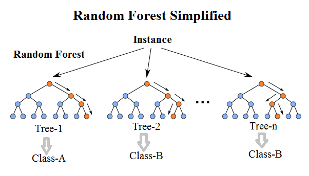
> Random Forest = Bagging + Decision Tree
---
**Ensemble Learning** a.k.a. 盲人摸象訓練術XD
有下列2種技巧,以面臨學校大考的例子說明。
**Bagging**
> 重複抽樣的概念。
> 狂買參考書來寫
**Boosting**
> 和bagging類似,但更注重改正錯誤
> 也是買參考書,但加強比較弱的、之寫寫錯的部分

---
參數說明:
1. **n_estimators**: 這個隨機森林裡面要包含幾棵決策樹?
> 100棵樹
2. **criterion**: 用來選決策樹的分割特徵的準則
> a. Gini Impurity
> b. Information Gain (by entropy) :heavy_check_mark:
3. 隨機打亂數據
> *seed = 42* 方便比較
```python=
from sklearn.ensemble import RandomForestClassifier
RandF = RandomForestClassifier(n_estimators = 100, criterion = 'entropy', random_state = 42)
RandF.fit(x_train_scaled, y_train_np)
```
---
### Cross Validation for Random Forest
**10-fold validation**
```python=
Kfold = model_selection.KFold(n_splits = 10, random_state = 42, shuffle = True)
scoring = 'accuracy' #我們要看交叉驗證的準確率如何
```
<br>驗證資料的準確率(accuracy)約為
> 99.1%
```python=
acc_RandF = cross_val_score(estimator = RandF, X = x_train_scaled, y = y_train_np, cv = Kfold, scoring = scoring)
acc_val = acc_RandF.mean()
print(acc_val)
```
<br>
---
### Model Evaluation for Random Forest
先求出真實答案&預測結果
```python=
ground_truth = y_test['Risk'].to_numpy()
predicted = RandF.predict(x_test_scaled)
```
<br>使用*sklearn*的現成函數計算performances
```python=
accuracy = accuracy_score(ground_truth, predicted)
precision = precision_score(ground_truth, predicted)
recall = recall_score(ground_truth, predicted)
F1 = f1_score(ground_truth, predicted)
ROC = roc_auc_score(ground_truth, predicted)
results_RandF = pd.DataFrame([['Random Forest', accuracy, acc_val, precision, recall, F1, ROC]], columns = ['Model', 'Accuracy','Cross Val Accuracy', 'Precision', 'Recall', 'F1 Score','ROC'])
results_RandF
```
<br>
隨機森林的表現近乎完美!訓練資料完全命中!
---
### K Nearest Neighbor (KNN) Algorithm

參數說明:**(都使用預設參數,未做更動)**
1. **n_neighbors**: $K$的大小,就是要參考附近幾個點?
> $K=5$
2. **weights**: 附近點的權重?
> 'uniform' (權重都均等)
3. **algorithm**: 使用的演算法
> a. brute force
> b. kd_tree
> c. ball_tree
> d. auto :heavy_check_mark:
4. **leaf_size**: kd樹或ball樹的大小
> 30 (default)
5. **p = 2**
> 歐式距離
6. **metric**: 度量距離的方式
> 'minkowski' (閔氏距離,就是p=2的歐式距離)
```python=
from sklearn.neighbors import KNeighborsClassifier
KNN = KNeighborsClassifier()
KNN.fit(x_train_scaled, y_train_np)
```
---
### Cross Validation for KNN
**10-fold validation**
```python=
Kfold = model_selection.KFold(n_splits = 10, random_state = 42, shuffle = True)
scoring = 'accuracy' #我們要看交叉驗證的準確率如何
```
<br>驗證資料的準確率(accuracy)約為
> 96.6%
```python=
acc_KNN = cross_val_score(estimator = KNN, X = x_train_scaled, y = y_train_np, cv = Kfold, scoring = scoring)
acc_val = acc_KNN.mean()
print(acc_val)
```
<br>
---
### Model Evaluation for KNN
先求出真實答案&預測結果
```python=
ground_truth = y_test['Risk'].to_numpy()
predicted = KNN.predict(x_test_scaled)
```
<br>使用*sklearn*的現成函數計算performances
```python=
accuracy = accuracy_score(ground_truth, predicted)
precision = precision_score(ground_truth, predicted)
recall = recall_score(ground_truth, predicted)
F1 = f1_score(ground_truth, predicted)
ROC = roc_auc_score(ground_truth, predicted)
results_KNN = pd.DataFrame([['K Nearest Neighbor', accuracy, acc_val, precision, recall, F1, ROC]], columns = ['Model', 'Accuracy','Cross Val Accuracy', 'Precision', 'Recall', 'F1 Score','ROC'])
results_KNN
```
<br>
雖不及隨機森林和羅吉斯回歸的效果,但仍然相當好,都有90%以上。
推測可能是因為只看附近的,所以效果上才不如前述兩者。
---
### Support Vector Machine (SVM)

參數說明:**(部分使用預設參數)**
1. **C**: 錯誤項的懲罰係數
越大訓練樣本越準,但泛化能力降低
> $C=1$ (default)
2. **kernel**: 核函數
可想像成把資料「投影」到更高維度,以方便分類的「投影函數」
> 'rbf' (default)
> 'linear' :heavy_check_mark:
3. **degree, gamma, coef0**: (略)
> 我們選擇linear kernel function,用不到這3個參數
4. **probability**: 是否啟用機率估計
> False (default)
> True :heavy_check_mark:
5. 隨機打亂數據
> *seed = 42* 方便比較
6. 其他參數保持預設,不一一列出
```python=
from sklearn.svm import SVC
SVM = SVC(kernel = "linear", probability = True, random_state = 42)
SVM.fit(x_train_scaled, y_train_np)
```
---
### Cross Validation for SVM
**10-fold validation**
```python=
Kfold = model_selection.KFold(n_splits = 10, random_state = 42, shuffle = True)
scoring = 'accuracy' #我們要看交叉驗證的準確率如何
```
<br>驗證資料的準確率(accuracy)約為
> 97.6%
```python=
acc_SVM = cross_val_score(estimator = SVM, X = x_train_scaled, y = y_train_np, cv = Kfold, scoring = scoring)
acc_val = acc_SVM.mean()
print(acc_val)
```
<br>
---
### Model Evaluation for SVM
先求出真實答案&預測結果
```python=
ground_truth = y_test['Risk'].to_numpy()
predicted = SVM.predict(x_test_scaled)
```
<br>使用*sklearn*的現成函數計算performances
```python=
accuracy = accuracy_score(ground_truth, predicted)
precision = precision_score(ground_truth, predicted)
recall = recall_score(ground_truth, predicted)
F1 = f1_score(ground_truth, predicted)
ROC = roc_auc_score(ground_truth, predicted)
results_SVM = pd.DataFrame([['Support Vector Machine', accuracy, acc_val, precision, recall, F1, ROC]], columns = ['Model', 'Accuracy','Cross Val Accuracy', 'Precision', 'Recall', 'F1 Score','ROC'])
results_SVM
```
<br>
結果略差於隨機森林,略好於KNN,和羅吉斯回歸差不多。
(RF > SVM $\approx$ LogReg > KNN)
仍然是相當不錯的分類表現,甚至都有超過95%。
---
### Neural Network

從**tensorflow**的**keras**匯入需要的方法,比如模型部分
```python=
from tensorflow.keras import backend as K
from tensorflow.keras.models import Sequential
from tensorflow.keras.layers import Dense
```
---
自定義計算精確率、召回率、F1分數的函式。(這部分參考老師的demo檔案)
```python=
def recall_m(y_true, y_pred):
true_positives = K.sum(K.round(K.clip(y_true * y_pred, 0, 1)))
possible_positives = K.sum(K.round(K.clip(y_true, 0, 1)))
recall = true_positives / (possible_positives + K.epsilon())
return recall
def precision_m(y_true, y_pred):
true_positives = K.sum(K.round(K.clip(y_true * y_pred, 0, 1)))
predicted_positives = K.sum(K.round(K.clip(y_pred, 0, 1)))
precision = true_positives / (predicted_positives + K.epsilon())
return precision
def f1_m(y_true, y_pred):
precision = precision_m(y_true, y_pred)
recall = recall_m(y_true, y_pred)
return 2*((precision*recall)/(precision+recall+K.epsilon()))
```
---
### 建造神經網路
1. 模型外面框架
```python=
NN = Sequential()
```
2. 輸入層(input layer):神經元個數 = 變數數量 = **15個**
```python=
x_train_scaled.shape
```

```python=
NN.add(Dense(16, activation = 'relu', input_shape = (x_train_scaled.shape[1], )))
```
3. 第一隱藏層(hidden layer): (程式碼請見上方)
> 16個神經元
> 激活函數(activation function): ***ReLU***
4. 第二隱藏層(hidden layer):
> 128個神經元
> 激活函數: ***ReLU***
```python=
NN.add(Dense(128, activation = 'relu'))
```
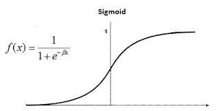
5. 輸出層(output layer)
> 只有**1**個神經元 → 給出預測結果
> 激活函數: ***Sigmoid*** → 因為是0或1的*二元預測*
---
### 組裝神經網路模型
```python=
NN.compile(optimizer = "rmsprop", loss = "binary_crossentropy", metrics = ['accuracy', recall_m, precision_m, f1_m])
```
> a. 優化器(optimizer): ***RMSProp***
> b. 損失函數(loss function): ***Binary Cross Entropy***
> c. 正確率衡量指標: 準確率***accuracy***、
自定義的召回率、精確率、F1分數***recall_m, precision_m, f1_m***
---
### 訓練神經網路
1. **20**個*epoch*
2. *batch大小* = **60**
> 約訓練資料集的1/10大小
```python=
history = NN.fit(x_train_scaled, y_train_np, epochs = 20, batch_size = 60)
```
訓練過程

---
### 查看每次epoch的表現(plot it out)
```python=
plt.figure(figsize = (25,5))
l = [
{'code':'loss',
'fullname':'Loss'},
{'code':'accuracy',
'fullname':'Accuracy'},
{'code':'precision_m',
'fullname':'Precision'},
{'code':'recall_m',
'fullname':'Recall'},
{'code':'f1_m',
'fullname':'F1 score'},
]
for i in range(5):
plt.subplot(1, 5, i+1).set_title("Model "+l[i]["fullname"])
plt.plot(history.history[l[i]["code"]])
plt.ylabel(l[i]["fullname"])
plt.xlabel("Epoch")
plt.tight_layout()
plt.savefig("NN_performance_plots.png")
```
<br>由左至右:**Loss, Accuracy, Precision, Recall, F1 score**

可以觀察到整體而言,損失有在下降,各項準確指標也有在上升。
雖然上升過程有些微不穩定。
四項準確指標都在約96-98%左右。
---
### Model Evaluation for Neural Network
下列evaluation時的指標,我自己刻程式計算
```python=
if m['type'] == 'Neural Network':
acc = (predicted == ground_truth).sum() / len(predicted)
precision = ground_truth[np.where(predicted == 1)].mean()
recall = predicted[np.where(ground_truth == 1)].mean()
F1 = 2 * precision * recall / (precision + recall)
print("accuracy:", acc)
print("precision:", precision)
print("recall:", recall)
print("F1:", F1)
print("AUC:", AUC)
```
<br>
---
### ROC曲線&曲線下面積AUC
使用*sklearn*套件中,*metrics*包裡面的現成方法**roc_curve, roc_auc_score**
```python=
from sklearn.metrics import roc_curve, roc_auc_score
```
<br>畫圖程式碼部分
```python=
y_test_np = y_test['Risk'].to_numpy()
models = [
{'type': 'Benchmark',
'model': 'Benchmark'},
{'type': 'Logistice Regression',
'model': LogisticRegression(random_state = 42, penalty = 'l1', solver='liblinear')},
{'type': 'Random Forest',
'model': RandomForestClassifier(n_estimators = 100, criterion = 'entropy', random_state = 42)},
{'type': 'K Nearest Neighbor',
'model': KNeighborsClassifier()},
{'type': 'Support Vector Machine',
'model': SVC(kernel = "linear", probability = True, random_state = 42)},
{'type': 'Neural Network',
'model': NN}
]
#預先設定整張圖大小
plt.figure(figsize = (20,10))
#算出每個模型的ROC和AUC,然後把曲線疊加到圖中
for m in models:
#我們需要特別處理我們手刻的benchmark,因為跟其他方法的結構不一樣,是自定義的
if m['type'] == 'Benchmark':
predicted = benchmark_test
#p = y.value_counts(normalize = True)[1],樣本中有審計風險的公司比例。約為39.3%
#n_test = len(x_test_scaled.index),縮放後測試資料集的長度
pred_prob = np.array([p] * n_test)
else:
model = m['model']
if m['type'] == 'Neural Network':
predicted = np.array([1 if model.predict(x_test_scaled)[i] >= 0.5 else 0 for i in range(len(model.predict(x_test_scaled)))], dtype = 'int64') #產生測試資料的預測結果(標籤)
pred_prob = model.predict(x_test_scaled) #產生測試資料預測出的,每筆資料的各標籤的機率
else:
model.fit(x_train_scaled, y_train_np) #訓練模型
predicted = model.predict(x_test_scaled) #產生測試資料的預測結果(標籤)
pred_prob = model.predict_proba(x_test_scaled)[:, 1] #產生測試資料預測出的,每筆資料的各標籤的機率
#計算真陽性率(TP rate)和偽陽性率(FP rate)
FP, TP, thresholds = roc_curve(y_test_np, pred_prob)
#計算AUC,然後呈現在ROC圖的legend中
AUC = roc_auc_score(y_test_np, predicted)
#接著,把結果疊加到ROC圖上
plt.plot(FP, TP, label = '%s ROC (area = %0.2f)' % (m['type'], AUC))
#一些圖片設定(標題、坐標軸標題等等)
plt.plot([0, 1], [0, 1], 'k--') #參考線
plt.xlim([0.0, 1.0]) #限制x軸顯示範圍
plt.ylim([0.0, 1.05]) #限制y軸顯示範圍
plt.xlabel('Specificity(FP rate)') #x軸標題
plt.ylabel('Sensitivity(TP rate)') #y軸標題
plt.title('ROC Figure') #圖片標題
plt.legend() #圖片圖例
plt.savefig("ROC.png") #儲存圖片
```
---
### 各模型ROC&AUC結果比較

---
### :star: **Results**
#### In-sample results (in percentage)
This is the accuracy for validation data.
|Measures |Benchmark Method|Logistic Regression|Random Forest|KNN|SVM|Neural Network|
|---|:---:|:---:|:---:|:---:|:---:|:---:|
| Accuracy |50.70|96.39|:crown: 99.14|96.56|97.59|97.77|
#### Out-of-sample comparisons (in percentage)
We consider a simple 75%-25% split on the data. In the test data, we have
|Measures |Benchmark Method|Logistic Regression|Random Forest|KNN|SVM|Neural Network|
|---|:---:|:---:|:---:|:---:|:---:|:---:|
| Accuracy |51.55|98.45|:crown:100|96.91|99.48|97.94|
| Precision|35.48|100|:crown:100|98.61|100|98.65|
| Recall |28.95|96.05|:crown:100|93.42|98.68|96.05|
|F1-score|31.88|97.99|:crown:100|95.95|99.34|97.33|
|AUC|47.52|98.03|:crown:100|96.29|99.34|97.60|
---
### :star: **Conclusion**
**Random Forest $>$ SVM $>$ Logistic Regression $>$ Neural Network $\gg$ KNN
$>>>>>>>>>>$ Benchmark Method**
所以我們應該選取***隨機森林(Random Forest)***,當作我們的二元預測模型。
---
### 混淆矩陣 (Confusion Matrix)
使用*sklearn*套件中,*metrics*包裡面的現成方法**confusion_matrix**
```python=
from sklearn.metrics import confusion_matrix
```
<br>畫圖程式碼部分
```python=
predicted = [
{'model': 'Benchmark Method',
'predicted': benchmark_test},
{'model': 'Logistice Regression',
'predicted': logReg.predict(x_test_scaled)},
{'model': 'Random Forest',
'predicted': RandF.predict(x_test_scaled)},
{'model': 'K Nearest Neighbor',
'predicted': KNN.predict(x_test_scaled)},
{'model': 'Support Vector Machine',
'predicted': SVM.predict(x_test_scaled)},
{'model': 'Neural Network',
'predicted': np.array([1 if NN.predict(x_test_scaled)[i] >= 0.5 else 0 for i in range(len(NN.predict(x_test_scaled)))], dtype = 'int64')}
]
plt.figure(figsize = (30, 20))
for i in range(len(predicted)):
cm = confusion_matrix(y_test_np, predicted[i]['predicted'])
plt.subplot(2, 3, i+1).set_title("Confusion Matrix of\n"+predicted[i]['model'])
sns.heatmap(cm, annot = True, fmt = 'd')
plt.savefig("Confusion_Matrixes.png")
#annot: annotation標上數字。
#fmt = 'd': 標上去的數字取整數
```
---
### 各模型混淆矩陣結果比較
從左上到右下:
> **Benchmark Method/ Logistic Regression/ Random Forest**
> **KNN/ SVM/ Neural Network**

可以發現所有模型都遠勝於Benchmark Method。
至於Benchmark Method外,其他5個模型之間的表現,請見***ROC&AUC***部分
---
### Feature Importances (for random forest)
1. Random Forest = 很多 Decision Tree
2. 每棵樹都會有自己挑選的辦法
> 對每棵樹而言,分類用到的變數不同,重要性也不同
#### Q: What is the overall influence for each variable?
---
使用到隨機森林分類器的內建屬性(attribute) -> ***feature_importances_***
```python=
importances = RandF.feature_importances_
indices = np.argsort(importances)[::-1]
#重新編排各個變數(特徵),使得他們對應到上面的這個重要性順序
features = [x.columns[i] for i in indices]
```
<br>畫圖部分程式碼
```python=
#創造一張空圖
plt.figure()
#圖片標題
plt.title("Feature Importances\n for Random Forest")
#加上每個特徵重要性的柱狀圖
#range(x.shape[1])代表所有0~行數-1
plt.bar(range(x.shape[1]), importances[indices])
#把每個特徵(變數)的名字標註到x軸
plt.xticks(range(x.shape[1]), features, rotation = 90)
#儲存圖片
plt.savefig("Feature Importances.png")
```
---
### 變數/特徵的重要性排序圖 (Feature Importance Plot)

可以看到最重要的分類特徵是變數**Inherent_Risk**,也就是說:
**總固有風險**部分,是判斷一個公司是否可能詐欺的一項重要指標。
---
## Future Works
如果能取得台灣公家企業(或普通企業)的風險分數資料,也可針對台灣的企業進行類似分析。
---
## 5. References
[我的資料來源 my dataset (from Kaggle)](https://www.kaggle.com/sid321axn/audit-data)
[參考論文:Fraudulent Firm Classification: A Case Study of an External Audit](https://www.researchgate.net/publication/323655455_Fraudulent_Firm_Classification_A_Case_Study_of_an_External_Audit)
[老師的demo檔案](https://drive.google.com/file/d/1C4tRbnbBhWcBpIsC4uaXkmbGBELegQPY/view?usp=sharing)
---
## 6. Data and Code Storage
Please refer to my E3.
---
 Sign in with Wallet
Connect another wallet
Sign in with Wallet
Connect another wallet