# WEEK 2
---
## TABLE OF CONTENT
[TOC]
---
## DAY 1
### Time Complexity
* Time complexity is a measurement of how much time an algorithm takes with respect to its input size.
* Big-O Notation is the most commonly used notation when discussing time complexity. The following are most commonly used when discussing time complexity:
* Constant time: $O(1)$
* Linear time: $O(n)$
* Quadratic: $O(n^2)$
* Exponential: $O(2^n)$
* Logarithmic: $O(log(n))$
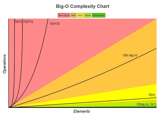
* We refer to the time complexity of an algorithm that has to check n elements as linear time.
* An algorithm with lower-order time complexities are more efficient. In other words, an algorithm of constant time is more efficient than linear time algorithms. Similarly, an algorithm which has $O(n^2)$ complexity is more efficient than an algorithm with $O(n^3)$ complexity.
### Helper Function: Timer
***Input***
```python
import functools
import time
import random
import math
def timer(func):
"""Print the runtime of the decorated function"""
@functools.wraps(func)
def wrapper_timer(*args, **kwargs):
start_time = time.perf_counter() # 1
value = func(*args, **kwargs)
end_time = time.perf_counter() # 2
run_time = end_time - start_time # 3
print(f"Finished {func.__name__!r} in {run_time:.6f} secs")
return value
return wrapper_timer
```
* **Example:**
***Input***
```python
def linear_search(a, x): # O(n)
"""Find the number x in list a.
Return -1 if not found"""
n = len(a)
for i in range(n):
if a[i] == x:
return i
return -1
n = n*10
a = [random.randrange(0, 100) for _ in range(n)]
%time linear_search(a,123)
```
***Output***
```python
CPU times: user 528 ms, sys: 0 ns, total: 528 ms
Wall time: 529 ms
-1
```
### Helper Function: Debuger
***Input***
```python
import functools
import time
import random
import math
def debug(func):
"""Print the function signature and return value"""
@functools.wraps(func)
def wrapper_debug(*args, **kwargs):
args_repr = [repr(a) for a in args] # 1
kwargs_repr = [f"{k}={v!r}" for k, v in kwargs.items()] # 2
signature = ", ".join(args_repr + kwargs_repr) # 3
print(f"Calling {func.__name__}({signature})")
value = func(*args, **kwargs)
print(f"{func.__name__!r} returned {value!r}") # 4
return value
return wrapper_debug
```
* **Example:**
***Input***
```python
@debug
def factorial(n):
"""Calculate n!
"""
if n == 1:
return 1
return n * factorial(n - 1)
factorial(5)
```
***Output***
```python
Calling factorial(5)
Calling factorial(4)
Calling factorial(3)
Calling factorial(2)
Calling factorial(1)
'factorial' returned 1
'factorial' returned 2
'factorial' returned 6
'factorial' returned 24
'factorial' returned 120
120
```
### Recursion (Recursive Function)
> A **recursive function** is a function that calls itself during its execution. The process may repeat several times, outputting the result and the end of each iteration.
* **Example 1:**
This is a simple example of recusion.


***Input***
```python
@debug
def factorial(n):
"""Calculate n!
"""
if n == 1:
return 1
return n * factorial(n - 1)
factorial(5)
```
***Output***
```python
Calling factorial(5)
Calling factorial(4)
Calling factorial(3)
Calling factorial(2)
Calling factorial(1)
'factorial' returned 1
'factorial' returned 2
'factorial' returned 6
'factorial' returned 24
'factorial' returned 120
120
```
* **Example 2:**
<img src="https://i.pinimg.com/originals/98/82/d5/9882d569f7e0b5665fe3b2edd5069b06.png" width="500">
<img src="https://miro.medium.com/max/500/1*AeRe16QGs8SJj7QP6zVrUw.png" width="300">
***Input***
```
@debug
def fib(n):
"""Calculate n!
"""
if (n==2) or (n==1):
return 1
return fib(n-1) + fib(n-2)
fib(4)
```
***Output***
```
Calling fib(4)
Calling fib(3)
Calling fib(2)
'fib' returned 1
Calling fib(1)
'fib' returned 1
'fib' returned 2
Calling fib(2)
'fib' returned 1
'fib' returned 3
3
```
### Sorting Algorithm
* Interactive sorting visualization: https://visualgo.net/bn/sorting
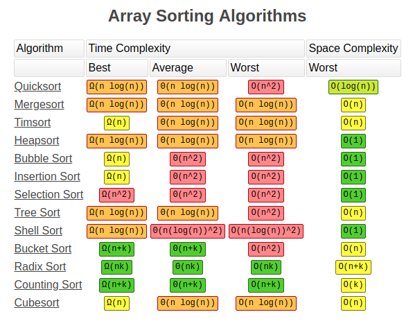
* **Bubble Sort**
> **Bubble Sort** compares adjacent elements of an array and organizes those elements. Its name comes from the fact that large numbers tend to “float” (bubble) to the top. It loops through an array and sees if the number at one position is greater than the number in the following position which would result in the number moving up. This cycle repeats until the algorithm has gone through the array without having to change the order
***Input***
```python
def bubble_sort(a): # O(N^2)
"""Sort the list a"""
n = len(a)
for j in range(n-1):
for i in range(n-1):
if a[i] > a[i+1]:
a[i], a[i+1] = a[i+1], a[i]
n = 50
a = [random.randrange(0, 100) for _ in range(n)]
print(a)
bubble_sort(a)
print(a)
```
***Output***
```python
[17, 37, 97, 24, 78, 15, 0, 79, 78, 99, 88, 46, 97, 50, 31, 28, 9, 93, 4, 83, 68, 28, 93, 5, 92, 52, 79, 30, 0, 71, 74, 19, 36, 87, 55, 96, 71, 60, 76, 73, 12, 2, 19, 55, 73, 18, 41, 11, 13, 14]
Finished 'bubble_sort' in 0.000444 secs
[0, 0, 2, 4, 5, 9, 11, 12, 13, 14, 15, 17, 18, 19, 19, 24, 28, 28, 30, 31, 36, 37, 41, 46, 50, 52, 55, 55, 60, 68, 71, 71, 73, 73, 74, 76, 78, 78, 79, 79, 83, 87, 88, 92, 93, 93, 96, 97, 97, 99]
```
* **Quick Sort**
> **Quicksort** is one of the most efficient sorting algorithms, and this makes of it one of the most used as well. The first thing to do is to select a pivot number, this number will separate the data, on its left are the numbers smaller than it and the greater numbers on the right. With this, we got the whole sequence partitioned. After the data is partitioned, we can assure that the partitions are oriented, we know that we have bigger values on the right and smaller values on the left.
***Input***
```python
def partition(a, low, high):
i = low - 1
pivot = a[high]
for j in range(low, high):
if a[j] <= pivot:
i = i + 1
a[i], a[j] = a[j], a[i]
a[high], a[i+1] = a[i+1], a[high]
return i+1
@debug
def quick_sort(a, low, high):
if low < high:
pivot = partition(a, low, high)
#print(a[low:pivot], a[pivot+1:high+1])
quick_sort(a, low, pivot -1)
quick_sort(a, pivot+1, high)
a = [10, 80, 90, 40, 50, 70]
quick_sort(a, 0, len(a)-1)
```
***Output***
```python
Calling quick_sort([10, 80, 90, 40, 50, 70], 0, 5)
Calling quick_sort([10, 40, 50, 70, 90, 80], 0, 2)
Calling quick_sort([10, 40, 50, 70, 90, 80], 0, 1)
Calling quick_sort([10, 40, 50, 70, 90, 80], 0, 0)
'quick_sort' returned None
Calling quick_sort([10, 40, 50, 70, 90, 80], 2, 1)
'quick_sort' returned None
'quick_sort' returned None
Calling quick_sort([10, 40, 50, 70, 90, 80], 3, 2)
'quick_sort' returned None
'quick_sort' returned None
Calling quick_sort([10, 40, 50, 70, 90, 80], 4, 5)
Calling quick_sort([10, 40, 50, 70, 80, 90], 4, 3)
'quick_sort' returned None
Calling quick_sort([10, 40, 50, 70, 80, 90], 5, 5)
'quick_sort' returned None
'quick_sort' returned None
'quick_sort' returned None
```
### Functional Programming
<img src="https://kingslanduniversity.com/wp-content/uploads/2019/04/functional_oo.png" width="500">
Functional programming emphasizes on **evaluation of functions**
- Functional programming provides the advantages like efficiency, lazy evaluation, nested functions, parallel programming. In simple language, **functional programming is to write the function having statements to execute a particular task for the application**
### Object Oriented Programming (OOP)
<img src="https://i.imgur.com/FgY1eRj.jpg" width="700">
<img src="https://topdev.vn/blog/wp-content/uploads/2019/05/class-object.png" width="700">
### Instance, Class, and Static Methods
**Build the simple object**
```python
class MyClass:
def method(self):
return 'instance method called', self
@classmethod
def classmethod(cls):
return 'class method called', cls
@staticmethod
def staticmethod():
return 'static method called'
```
> **Example 1: Create instance and call the instance method**
***Call Instance method***
```python
>>> obj = MyClass()
>>> obj.method()
('instance method called', <MyClass instance at 0x10205d190>)
```
```python
>>> MyClass.method(obj)
('instance method called', <MyClass instance at 0x10205d190>)
```
***Call Class method***
```python
>>> obj.classmethod()
('class method called', <class MyClass at 0x101a2f4c8>)
```
***Call Static method***
```python
>>> obj.staticmethod()
'static method called'
```
> **Example 2: Call methods without creating an object instance beforehand:**
```python
>>> MyClass.classmethod()
('class method called', <class MyClass at 0x101a2f4c8>)
>>> MyClass.staticmethod()
'static method called'
>>> MyClass.method()
TypeError: unbound method method() must
be called with MyClass instance as first
argument (got nothing instead)
```
We **were able to call classmethod() and staticmethod()** just fine, but attempting to **call the instance method method() failed with a TypeError**.
And this is to be expected — this time we didn’t create an object instance and tried calling an instance function directly on the class blueprint itself. This means there is no way for Python to populate the self argument and therefore the call fails.
* ***Instance methods*** need a class instance and can access the instance through self.
* ***Class methods*** don’t need a class instance. They can’t access the instance (self) but they have access to the class itself via cls.
* ***Static methods*** don’t have access to cls or self. They work like regular functions but belong to the class’s namespace.
* ***Static and class methods*** communicate and (to a certain degree) enforce developer intent about class design. This can have maintenance benefits.
---
## DAY 2
### NumPy stands for Numerical Python
* NumPy is, just like SciPy, Scikit-Learn, Pandas, etc. one of the packages that you just can’t miss when you’re learning data science, mainly because this library provides you with an array data structure that holds some benefits over Python lists, such as: being more compact, faster access in reading and writing items, being more convenient and more efficient.
* NumPy is constrained to arrays that all contain the same type. If types do not match, NumPy will upcast if possible (here, integers are up-cast to floating point)
<img src="https://i.imgur.com/VSCCjUx.png" width="650">
***Input 1:***
```python
# Create a 2d array with 1 on the border and 0 inside
a = np.ones(shape=(10,10))
a[1:-1,1:-1] = 0
print(a)
```
***Output 1:***
```python
[[1. 1. 1. 1. 1. 1. 1. 1. 1. 1.]
[1. 0. 0. 0. 0. 0. 0. 0. 0. 1.]
[1. 0. 0. 0. 0. 0. 0. 0. 0. 1.]
[1. 0. 0. 0. 0. 0. 0. 0. 0. 1.]
[1. 0. 0. 0. 0. 0. 0. 0. 0. 1.]
[1. 0. 0. 0. 0. 0. 0. 0. 0. 1.]
[1. 0. 0. 0. 0. 0. 0. 0. 0. 1.]
[1. 0. 0. 0. 0. 0. 0. 0. 0. 1.]
[1. 0. 0. 0. 0. 0. 0. 0. 0. 1.]
[1. 1. 1. 1. 1. 1. 1. 1. 1. 1.]]
```
***Input 2:***
```python
# Create a 2d identity matrix:
a = np.eye(5)
print(a)
```
***Output 2:***
```python
[[1. 0. 0. 0. 0.]
[0. 1. 0. 0. 0.]
[0. 0. 1. 0. 0.]
[0. 0. 0. 1. 0.]
[0. 0. 0. 0. 1.]]
```
***Input 3:***
```python
# Create a constant array
a = np.full((5,5), 7)
print(a)
```
***Output 3:***
```python
[[7 7 7 7 7]
[7 7 7 7 7]
[7 7 7 7 7]
[7 7 7 7 7]
[7 7 7 7 7]]
```
***Input 4:***
```python
# Create an array of random number
a = np.random.random((3,3))
print(a)
```
***Output 4:***
```python
[[0.85505308 0.21635304 0.84760135]
[0.58465946 0.64834319 0.5316686 ]
[0.08053296 0.4956883 0.77956674]]
```
### Index in NumPy
<div align="left">
<img src="https://i.imgur.com/y0CL0S4.png" width="300">
</div>
***Input***
```python
x = np.array([[1,2,3,4], [5,6,7,8], [9,10,11,12]])
print (x)
print ("indexed values: \n", x[[0,1,2], [0,2,1]])
print ("x rows 0,1 & cols 1,2: \n", x[0:2, 1:3])
```
***Output:***
```python
[[ 1 2 3 4]
[ 5 6 7 8]
[ 9 10 11 12]]
indexed values:
[ 1 7 10]
x rows 0,1 & cols 1,2:
[[2 3]
[6 7]]
```
### Dot Product in NumPy
<div align="left">
<img src="https://raw.githubusercontent.com/madewithml/images/master/basics/03_NumPy/dot.gif" width="450">
</div>
### Axis operation
<div align="left">
<img src="https://raw.githubusercontent.com/madewithml/images/master/basics/03_NumPy/axis.gif" width="450">
</div>
* Sum across dimension
***Input:***
```python
# Sum across a dimension
x = np.array([[1,2,3,4],[1,2,3,4],[1,2,3,4]])
print (x)
print (x.shape)
print ("sum all: ", np.sum(x)) # adds all elements
print ("sum axis=0: ", np.sum(x, axis=0)) # sum across rows
print ("sum axis=1: ", np.sum(x, axis=1)) # sum across columns
```
***Output:***
```python
[[1 2 3 4]
[1 2 3 4]
[1 2 3 4]]
(3, 4)
sum all: 30
sum axis=0: [ 3 6 9 12]
sum axis=1: [10 10 10]
```
* Min/max across dimension
***Input:***
```python
# Min/max
x = np.array(
[[1,2,3],
[44,45,0]]
)
print(x)
print(x.shape)
print ("min: ", x.min())
print ("max: ", x.max())
print ("min axis=0: ", x.min(axis=0))
print ("min axis=1: ", x.min(axis=1))`
```
***Output:***
```python
[[ 1 2 3]
[44 45 0]]
(2, 3)
min: 0
max: 45
min axis=0: [1 2 0]
min axis=1: [1 0]
```
### Transposing
To transpose a matrix there are two steps:
1. Rotate the matrix 90°
2. Reverse the order of elements in each row (e.g. [a b ] becomes [b a])
<div align="left">
<img src="https://raw.githubusercontent.com/madewithml/images/master/basics/03_NumPy/transpose.png" width="400">
</div>
***Input:***
```python
x = np.array([[1,2,3], [4,5,6]])
print ("x:\n", x)
print ("x.shape: ", x.shape)
x_transpose= x.T
print ("X transpose:\n", x_transpose)
print ("X.T shape: ", x_transpose.shape)
```
***Output:***
```python
x:
[[1 2 3]
[4 5 6]]
x.shape: (2, 3)
X transpose:
[[1 4]
[2 5]
[3 6]]
X.T shape: (3, 2)
```
### Reshape
**Reshaping allows us to transform a tensor into different permissible shapes** -- our reshaped tensor has the same amount of values in the tensor. (1X6 = 2X3).**We can also use `-1` on a dimension and NumPy will infer the dimension based on our input tensor.**
The way reshape works is by looking at each dimension of the new tensor and separating our original tensor into that many units. So here the dimension at index 0 of the new tensor is 2 so we divide our original tensor into 2 units, and each of those has 3 values.
<div align="left">
<img src="https://raw.githubusercontent.com/madewithml/images/master/basics/03_NumPy/reshape.png" width="450">
</div>
### Broadcasting
The scalar is ***broadcast*** across the vector so that they have compatible shapes.
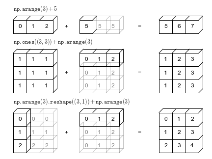
Broadcasting in NumPy follows a strict set of rules to determine the interaction between the two arrays:
When operating on two arrays, NumPy compares their shapes element-wise.
- Step 1: If the two arrays differ in their number of dimensions, the shape of the one with fewer dimensions is padded with ones on its leading (left) side.
- Step 2: We **starts with the trailing (most right) dimensions and works its way to the left**. Two dimensions are compatible when
- they are equal, or
- one of them is 1
---
## DAY 3
### What is Database?
A database is a set of data stored in a computer. This data is usually structured in a way that makes the data easily accessible. Type of database:
- Relational Database
- Non-relational Database or NO-SQL Database
### What is Relational Database?
A realtional database is a type of database. The relational database organizes data into tables which can be linked—or **related**—based on data common to each.
- **Table** (Entity): A structured list of data.
- **Column**: A table is made up of one or more columns. Each of the column have a specific data type.
- **Row** (Record): a table can have multiple row.
- **Primary key**: a column that uniquely identifies each row in a table
- No two rows can have the same primary key value
- Every row must have a value in the primary key column(s).
- Values in primary key columns should never be modified or updated.
- Primary key values should never be reused.
- **Foreign Key**: a referencing key that's used to link two tables together. It could be a column or combination of columns whose values match a Primary Key in a different table.
### What is Non Relational Database?
Non-relational databases (often called NoSQL databases) are different from traditional relational databases in that they store their data in a **non-tabular** form. Instead, non-relational databases might be **based on data structures like documents**. A document can be highly detailed while containing a range of different types of information in different formats. This ability to digest and organize various types of information side-by-side makes **non-relational databases much more flexible than relational databases**.
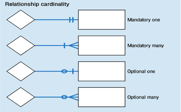
### What is Entity Relationship Diagram (ERD) ?
ERD displays the relationships of table (entity) set stored in a database. In other words, we can say that ER diagrams help you to explain the logical structure of databases. It is considered a best practice to complete ERD before implementing your database. Because the ERD will provide a preview of how all your tables should connect, what fields are going to be on each table, this will help you produce a well-designed database.
- Different types of entity relationships are:
- One-to-One Relationships
- One-to-Many Relationships
- Many to One Relationships
- Many-to-Many Relationships
### Operator in SQL
| Operator | Condition | SQL Example |
|:--------------:|:---------------:|:----------------------:|
| =, !=, < <=, >, >= | Standard numerical operators | col_name != 4 |
| **BETWEEN** … **AND** … | Number is within range of two values (inclusive) | col_name **BETWEEN** 1.5 **AND** 10.5 |
| **NOT BETWEEN** … **AND** … | Number is not within range of two values (inclusive) | col_name **NOT BETWEEN** 1 **AND** 10 |
| **IN** (…) | Number exists in a list | col_name **IN** (2, 4, 6) |
| **NOT IN** (…) | Number does not exist in a list | col_name **NOT IN** (1, 3, 5) |
| Operator | Condition | SQL Example |
|:--------------:|:---------------:|:----------------------:|
| = | Case sensitive exact string comparison (notice the single equals) | col_name = "abc" |
| != or <> | Case sensitive exact string inequality comparison | col_name != "abcd" |
| **LIKE** | Case insensitive exact string comparison | col_name **LIKE** "ABC" |
| **NOT LIKE** | Case insensitive exact string inequality comparison | col_name **NOT LIKE** "ABCD" |
| % | Used anywhere in a string to match a sequence of zero or more characters (only with **LIKE** or **NOT LIKE**) | col_name **LIKE** "%AT%" (matches "AT", "ATTIC", "CAT" or even "BATS") |
| _ | Used anywhere in a string to match a single character (only with **LIKE** or **NOT LIKE**) | col_name **LIKE** "AN_" (matches "AND", but not "AN") |
| **IN** (…) | String exists in a list | col_name **IN** ("A", "B", "C") |
| **NOT IN** (…) | String does not exist in a list | col_name **NOT IN** ("D", "E", "F") |
### SQL Query
***SELECT***
```sql
SELECT column, another_column, …
FROM mytable;
```
***SELECT with condition***
```sql
SELECT column_1, column_2, ...
FROM mytable
WHERE conditions
AND/OR another_condition
AND/OR ...;
```
***ORDER BY***
```sql
SELECT column_1, column_2, …
FROM mytable
WHERE condition(s)
ORDER BY column_3 ASC/DESC;
```
***LIMIT and OFFSET***
```sql
SELECT column_1, column_2, …
FROM mytable
WHERE condition(s)
ORDER BY column_3 ASC/DESC
LIMIT num_limit OFFSET num_offset;
```
***JOIN***
```sql
SELECT mytable.column_1, mytable.column_2, another_table.column_1, ....
FROM mytable
INNER JOIN another_table
ON mytable.id = another_table.id
WHERE condition(s)
ORDER BY mytable.column_4, … ASC/DESC
LIMIT num_limit OFFSET num_offset;
```
### INNER JOIN, LEFT JOIN, RIGHT JOIN, FULL OUTER JOIN
* The **INNER JOIN** is a process that matches rows from the first table and the second table which have the same key (as defined by the **ON** constraint) to create a result row with the combined columns from both tables.
* If the two tables have asymmetric data, which can easily happen when data is entered in different stages, then we would have to use a **LEFT JOIN**, **RIGHT JOIN** or **FULL JOIN** instead **to ensure that the data you need is not left out of the results.**
```sql
SELECT mytable.column, another_table.another_column, …
FROM mytable
INNER/LEFT/RIGHT/FULL JOIN another_table
ON mytable.id = another_table.matching_id
WHERE condition(s)
ORDER BY column, … ASC/DESC
LIMIT num_limit OFFSET num_offset;
```
* Sometimes, it's not possible to avoid **NULL** values. In these case, you can test a column for **NULL** values in a WHERE clause by using either the **IS NULL** or **IS NOT NULL** constraint.
```sql
SELECT mytable.column, another_table.another_column, …
FROM mytable
WHERE column IS/IS NOT NULL
AND/OR another_condition
AND/OR …;
```
### GROUP BY
```sql
SELECT AGG_FUNC(column_or_expression) AS aggregate_description, …
FROM mytable
WHERE constraint_expression
GROUP BY column;
```
### GROUP BY with condition
```sql
SELECT group_by_column, AGG_FUNC(column_expression) AS aggregate_result_alias, …
FROM mytable
WHERE condition
GROUP BY column
HAVING group_condition;
```
### Aggregates function
| Functions | Description |
|:-:|:-:|
|**COUNT**(\*), **COUNT**(column) | A common function used to counts the number of rows in the group if no column name is specified. Otherwise, count the number of rows in the group with non-NULL values in the specified column.|
|**MIN**(column) | Finds the smallest numerical value in the specified column for all rows in the group.|
|**MAX**(column) | Finds the largest numerical value in the specified column for all rows in the group.|
|**AVG**(column) | Finds the average numerical value in the specified column for all rows in the group.|
|**SUM**(column) | Finds the sum of all numerical values in the specified column for the rows in the group.|
### Query order of execution
Now that we have an idea of all the parts of a query, we can now talk about how they all fit together in the context of a complete query.
1. **FROM** and **JOIN**
2. **WHERE**
3. **GROUP BY**
4. **HAVING**
5. **SELECT**
6. **DISTINCT**
7. **ORDER BY**
8. **LIMIT** / **OFFSET**
---
## DAY 4
### Sub-queries
Sub-queries are SQL queries nested inside a larger query.
```sql
SELECT column_names
FROM table_names
WHERE condition IN
(SELECT column_names
FROM other_table
WHERE condition)
```
### Common table expression (CTE)
- Provide a teporary result (temp table) to use with other queries
- Help organize complex queries
```sql
WITH table_temp AS
(SELECT t1.column1, t2.column2
FROM table_1 AS t1 JOIN table_2 AS t2
ON t1.column3 = t2.column4)
SELECT *
FROM table_temp
```
### Set Operators
Set Operators allow the results multiple queries to be combined together.
```sql
SELECT col1, col2
FROM table1
UNION / UNION ALL / INTERSECT / EXCEPT
SELECT col1, col2
FROM table2
```
 Sign in with Wallet
Connect another wallet
Sign in with Wallet
Connect another wallet