# Release Highlights for scikit-learn 0.24(翻譯)
###### tags: `scikit-learn` `sklearn` `python` `machine learning` `Release Highlights` `翻譯`
[原文連結](https://scikit-learn.org/stable/auto_examples/release_highlights/plot_release_highlights_0_24_0.html)
我們很高興宣佈scikit-learn 0.24的發布,其中包含許多bug的修復以及新功能!下面我們詳細說明這版本的一些主要功能。關於完整的修正清單,請參閱[發行說明](https://scikit-learn.org/stable/whats_new/v0.23.html#changes-0-23)。
安裝最新版本(使用pip):
```shell
pip install --upgrade scikit-learn
```
或者使用conda:
```shell
conda install -c conda-forge scikit-learn
```
:::info
## Successive Halving estimators for tuning hyper-parameters
:::
Successive Halving,當前最好的方法,現在可以用來探索參數空間並確定它們的最佳組合。[HalvingGridSearchCV](https://scikit-learn.org/stable/modules/generated/sklearn.model_selection.HalvingGridSearchCV.html#sklearn.model_selection.HalvingGridSearchCV)與[HalvingRandomSearchCV](https://scikit-learn.org/stable/modules/generated/sklearn.model_selection.HalvingRandomSearchCV.html#sklearn.model_selection.HalvingRandomSearchCV)可以直接拿來替代 [GridSearchCV](https://scikit-learn.org/stable/modules/generated/sklearn.model_selection.GridSearchCV.html#sklearn.model_selection.GridSearchCV)and[RandomizedSearchCV](https://scikit-learn.org/stable/modules/generated/sklearn.model_selection.RandomizedSearchCV.html#sklearn.model_selection.RandomizedSearchCV)。Successive Halving是一種迭代選擇的過程,如下圖所示。第一次的迭代會用少許的資源來執行,通常資源取決於訓練樣本的數量,但也可以是任意整數參數,像是隨機森林中的`n_estimators`。只會選擇候選參數的子集來用於下一次的迭代,而下一次的迭代會在分配資源增加的情況下執行。只會有一部份的候選參數會持續到迭代過程的最後,而最佳參數候選就會是在最後一次迭代中得分最高的那一個。
更多可參閱[使用者指南](https://scikit-learn.org/stable/modules/grid_search.html#successive-halving-user-guide)(注意到,Successive Halving estimators仍然是[實驗性質的](https://scikit-learn.org/stable/glossary.html#term-experimental)。)

圖片來自[Scikit-learn](https://scikit-learn.org/)官方
```python
import numpy as np
from scipy.stats import randint
from sklearn.experimental import enable_halving_search_cv # noqa
from sklearn.model_selection import HalvingRandomSearchCV
from sklearn.ensemble import RandomForestClassifier
from sklearn.datasets import make_classification
rng = np.random.RandomState(0)
X, y = make_classification(n_samples=700, random_state=rng)
clf = RandomForestClassifier(n_estimators=10, random_state=rng)
param_dist = {"max_depth": [3, None],
"max_features": randint(1, 11),
"min_samples_split": randint(2, 11),
"bootstrap": [True, False],
"criterion": ["gini", "entropy"]}
rsh = HalvingRandomSearchCV(estimator=clf, param_distributions=param_dist,
factor=2, random_state=rng)
rsh.fit(X, y)
rsh.best_params_
```
:::info
## Native support for categorical features in HistGradientBoosting estimators
:::
HistGradientBoostingClassifier與HistGradientBoostingRegressor現在對類別屬性的特徵有原生支援:它們可以考慮對無序的分類資料做拆分。更多請參考[使用者指南](https://scikit-learn.org/stable/modules/ensemble.html#categorical-support-gbdt)。

圖片來自[Scikit-learn](https://scikit-learn.org/)官方
此圖說明了對類別屬性的特徵新的原生支援對比處理過的(像是簡單的序數編碼)類別屬性特徵所導致的擬合時間。原生支援比起one-hot encoding與ordinal encoding表現更好。但是,要使用新的參數`categorical_features`之前,不免的還需要對pipeline裡面的資料做前置預處理,見[範例](https://scikit-learn.org/stable/auto_examples/ensemble/plot_gradient_boosting_categorical.html#sphx-glr-auto-examples-ensemble-plot-gradient-boosting-categorical-py)說明。
:::info
## Improved performances of HistGradientBoosting estimators
:::
[ensemble.HistGradientBoostingRegressor](https://scikit-learn.org/stable/modules/generated/sklearn.ensemble.HistGradientBoostingRegressor.html#sklearn.ensemble.HistGradientBoostingRegressor)與[ensemble.HistGradientBoostingClassifier](https://scikit-learn.org/stable/modules/generated/sklearn.ensemble.HistGradientBoostingClassifier.html#sklearn.ensemble.HistGradientBoostingClassifier)的記憶體耗用量在呼叫`fit`期間明顯的改善。此外,現在直方圖的初始化可以並行完成,速度有些許的提升。更多請參閱[基準頁面](https://scikit-learn.org/scikit-learn-benchmarks/)。
:::info
## New self-training meta-estimator
:::
一種新的self-training實現,基於[Yarowski’s algorithm](https://dl.acm.org/doi/10.3115/981658.981684),可以搭配任意的分類器(該分類器必需有實作[predict_proba](https://scikit-learn.org/stable/glossary.html#term-predict_proba))。子分類器會表現的像是一個半監督的分類器(semi-supervised classifier),允許從未標記資料中學習。更多請參閱[使用者指南](https://scikit-learn.org/stable/modules/semi_supervised.html#self-training)。
```python
import numpy as np
from sklearn import datasets
from sklearn.semi_supervised import SelfTrainingClassifier
from sklearn.svm import SVC
rng = np.random.RandomState(42)
iris = datasets.load_iris()
random_unlabeled_points = rng.rand(iris.target.shape[0]) < 0.3
iris.target[random_unlabeled_points] = -1
svc = SVC(probability=True, gamma="auto")
self_training_model = SelfTrainingClassifier(svc)
self_training_model.fit(iris.data, iris.target)
```
:::info
## New SequentialFeatureSelector transformer
:::
一個用於選擇特徵的迭代轉換器閃亮亮登場:[SequentialFeatureSelector](https://scikit-learn.org/stable/modules/generated/sklearn.feature_selection.SequentialFeatureSelector.html#sklearn.feature_selection.SequentialFeatureSelector)。Sequential Feature Selector可以一次增加一個特徵(前向選擇)或從可用特徵列表中移除一個特徵(反向選擇),基於交叉驗證分數最大化。見[使用者指南](https://scikit-learn.org/stable/modules/feature_selection.html#sequential-feature-selection)。
```python
from sklearn.feature_selection import SequentialFeatureSelector
from sklearn.neighbors import KNeighborsClassifier
from sklearn.datasets import load_iris
X, y = load_iris(return_X_y=True, as_frame=True)
feature_names = X.columns
knn = KNeighborsClassifier(n_neighbors=3)
sfs = SequentialFeatureSelector(knn, n_features_to_select=2)
sfs.fit(X, y)
print("Features selected by forward sequential selection: "
f"{feature_names[sfs.get_support()].tolist()}")
```
:::warning
Out: Features selected by forward sequential selection: ['petal length (cm)', 'petal width (cm)']
:::
:::info
## New PolynomialCountSketch kernel approximation function
:::
新的[PolynomialCountSketch](https://scikit-learn.org/stable/modules/generated/sklearn.kernel_approximation.PolynomialCountSketch.html#sklearn.kernel_approximation.PolynomialCountSketch)近似特徵空間的多項式擴展(與線性模型搭配使用的時候),但記憶體用量較[PolynomialFeatures](https://scikit-learn.org/stable/modules/generated/sklearn.preprocessing.PolynomialFeatures.html#sklearn.preprocessing.PolynomialFeatures)還要少。
```python
from sklearn.datasets import fetch_covtype
from sklearn.pipeline import make_pipeline
from sklearn.model_selection import train_test_split
from sklearn.preprocessing import MinMaxScaler
from sklearn.kernel_approximation import PolynomialCountSketch
from sklearn.linear_model import LogisticRegression
X, y = fetch_covtype(return_X_y=True)
pipe = make_pipeline(MinMaxScaler(),
PolynomialCountSketch(degree=2, n_components=300),
LogisticRegression(max_iter=1000))
X_train, X_test, y_train, y_test = train_test_split(X, y, train_size=5000,
test_size=10000,
random_state=42)
pipe.fit(X_train, y_train).score(X_test, y_test)
```
:::warning
Out: 0.7336
:::
做為比較,這邊給出使用相同資料情況下,其線性基線的分數:
```python
linear_baseline = make_pipeline(MinMaxScaler(),
LogisticRegression(max_iter=1000))
linear_baseline.fit(X_train, y_train).score(X_test, y_test)
```
:::warning
Out: 0.7137
:::
:::info
## Individual Conditional Expectation plots
:::
一種新的部份相依圖(PDP):個體條件期望圖(ICE)(顯示對於每一個樣本實例,當改變某一個特徵值的時候,預測結果會如何改變。)。ICE圖各別可視化在特徵上對每一個樣本預測的相依性,每個樣本一行。見[使用者指南](https://scikit-learn.org/stable/modules/partial_dependence.html#individual-conditional)。
```python
from sklearn.datasets import fetch_california_housing
from sklearn.inspection import plot_partial_dependence
X, y = fetch_california_housing(return_X_y=True, as_frame=True)
features = ['MedInc', 'AveOccup', 'HouseAge', 'AveRooms']
est = RandomForestRegressor(n_estimators=10)
est.fit(X, y)
display = plot_partial_dependence(
est, X, features, kind="individual", subsample=50,
n_jobs=3, grid_resolution=20, random_state=0
)
display.figure_.suptitle(
'Partial dependence of house value on non-location features\n'
'for the California housing dataset, with BayesianRidge'
)
display.figure_.subplots_adjust(hspace=0.3)
```
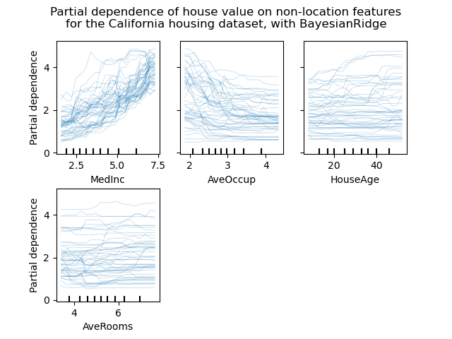
圖片來自[Scikit-learn](https://scikit-learn.org/)官方
:::info
## New Poisson splitting criterion for DecisionTreeRegressor
:::
The integration of Poisson regression estimation continues from version 0.23.
[DecisionTreeRegressor](https://scikit-learn.org/stable/modules/generated/sklearn.tree.DecisionTreeRegressor.html#sklearn.tree.DecisionTreeRegressor)現在支援一個新的`poisson`分割標準。如果你的目標是計數或頻率,那設置`criterion="poisson"`也許是一個不錯的選擇。
```python
from sklearn.tree import DecisionTreeRegressor
from sklearn.model_selection import train_test_split
import numpy as np
n_samples, n_features = 1000, 20
rng = np.random.RandomState(0)
X = rng.randn(n_samples, n_features)
# positive integer target correlated with X[:, 5] with many zeros:
y = rng.poisson(lam=np.exp(X[:, 5]) / 2)
X_train, X_test, y_train, y_test = train_test_split(X, y, random_state=rng)
regressor = DecisionTreeRegressor(criterion='poisson', random_state=0)
regressor.fit(X_train, y_train)
```
:::info
## New documentation improvements
:::
為了不斷提升對機器學一得理解,我們已經著手增加新的範例與文件頁面:
* 新的章節關於[常見陷阱與建議作法](https://scikit-learn.org/stable/common_pitfalls.html#common-pitfalls)
* 範例說明如何統計比較使用[GridSerchCV](https://scikit-learn.org/stable/modules/generated/sklearn.model_selection.GridSearchCV.html#sklearn.model_selection.GridSearchCV)來[評估模型效能](https://scikit-learn.org/stable/auto_examples/model_selection/plot_grid_search_stats.html#sphx-glr-auto-examples-model-selection-plot-grid-search-stats-py)
* 範例說明如何解釋[線性模型的係數](https://scikit-learn.org/stable/auto_examples/inspection/plot_linear_model_coefficient_interpretation.html#sphx-glr-auto-examples-inspection-plot-linear-model-coefficient-interpretation-py)
* [範例](https://scikit-learn.org/stable/auto_examples/cross_decomposition/plot_pcr_vs_pls.html#sphx-glr-auto-examples-cross-decomposition-plot-pcr-vs-pls-py)比較Principal Component Regression(PCA,主成份回歸)與Partial Least Squares(PLS,偏最小平方法)
 Sign in with Wallet
Connect another wallet
Sign in with Wallet
Connect another wallet