# 機器學習基礎
By. RoyChuang
<!-- Special Thanks to [**lucasw**](https://slides.com/lucasw) and [**NTUEE李宏毅教授**](https://speech.ee.ntu.edu.tw/~hylee/ml/2016-fall.php) ~~因為大部分的圖都是這邊偷來的~~
-->
## 背景
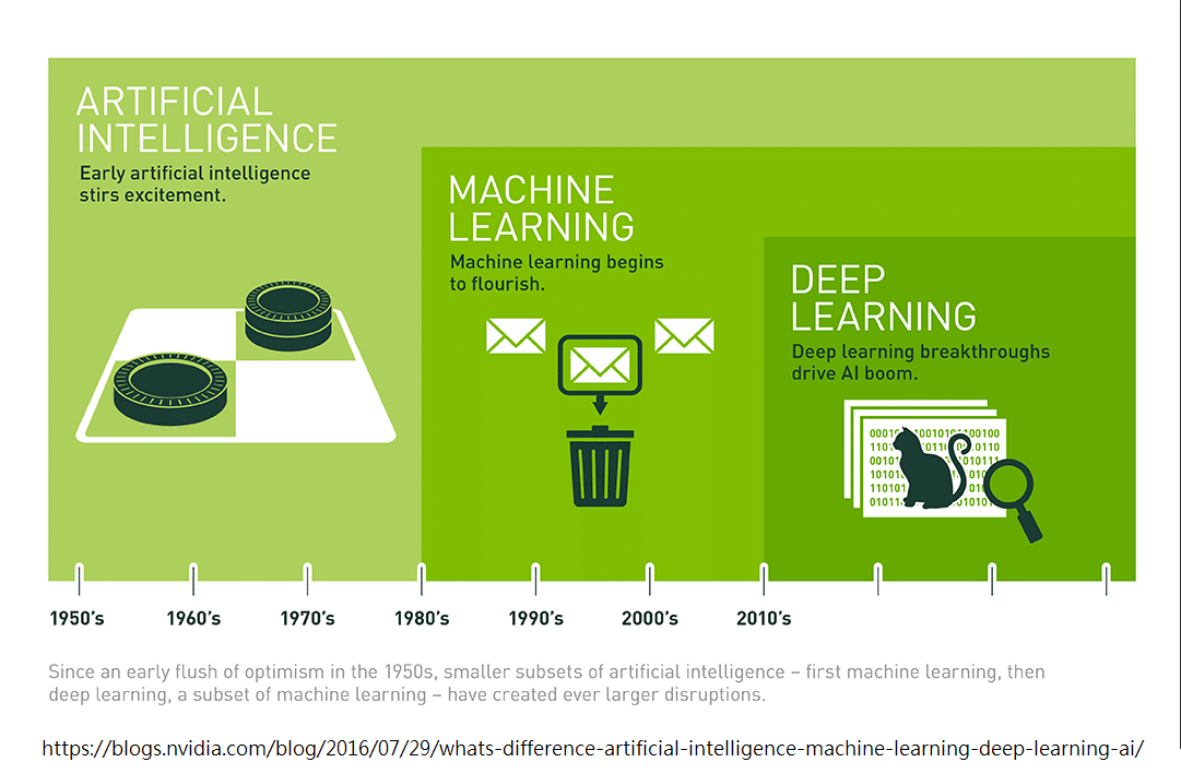
**人工智慧 (artificial intelligence, AI)** ,由**愛倫·圖靈 (Alan Turing)** 所提出的概念,代表使用電腦去模擬人類具有智慧的行為,例如**語言、學習、思考、論證、創造**等等。
**機器學習 (Machine Learning, ML)**,1959 年被 IBM 員工 **Arthur Samuel** 提出,代表透過統計學,讓機器自己做學習,而並非用一條指令一個動作的方式,來製造人工智慧。
**深度學習 (Deep Learning)**,一種機器學習的方法,我們模擬人類大腦神經元的運作模式,由許多神經細胞構成神經網路,經歴學習的過程,藉此訓練一個 AI。
深度學習又可以分為 **Multilayer perceptron (MLP)**, **Recurrent neural network (RNN)**, **convolutional neural network (CNN)** 等等。
今天會講最基礎的 MLP。
## 深度學習的原理
### 人類大腦的運作原理
<blockquote>
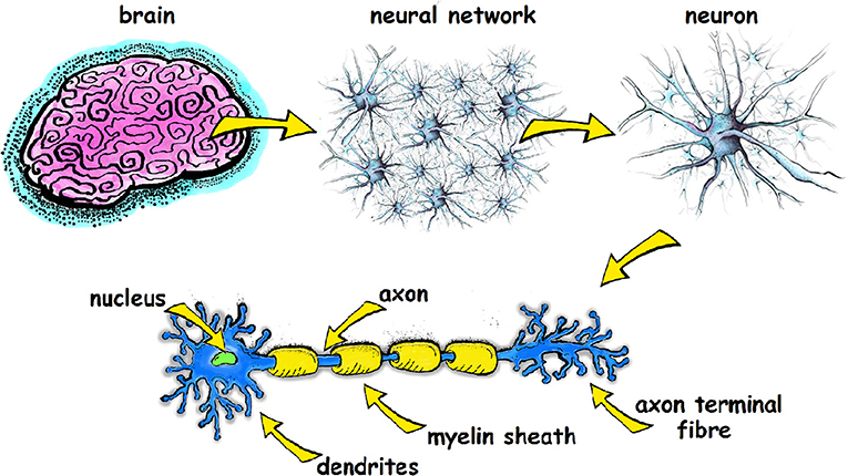
大腦裡有大約 860 億個神經元。每個神經元都像一個小小的訊號處理器,負責「接收 → 判斷 → 傳送」訊息。
神經元彼此不是直接黏在一起,而是隔著一點點縫隙,這個縫隙叫做突觸。
當你看到、聽到、想到某件事時,神經元會先用**電訊號**在自己體內傳遞;到了突觸,就改用**化學物質(神經傳導物質)** 把訊息丟給下一個神經元。
一個神經元通常同時接收「很多」其他神經元的訊號,它會把這些訊號加總、比較,如果強度夠大,就觸發下一次放電。這個「是否觸發」的過程,就是最基本的「判斷」。
所謂的「思考」,不是單一神經元在想事情,而是:
- 大量神經元同時活動
- 訊號在特定路徑中反覆流動
某些連線被用得越多,突觸就會變得越強(這就是學習與記憶的基礎)
所以:
- 想一個數學題 → 某些神經網路被啟動
- 回憶一段音樂 → 另一組神經連線被重播
- 情緒影響判斷 → 情緒相關的神經區域改變訊號權重
一句話總結:
**人類的思考,是神經元用電與化學訊號,在不斷變化的連線網路中進行大規模「加權傳遞」的結果。**
-- ChatGPT
</blockquote>
<center><small> 圖取自frontiersin.org </small></center>
---
### 類神經網路
<!--  -->
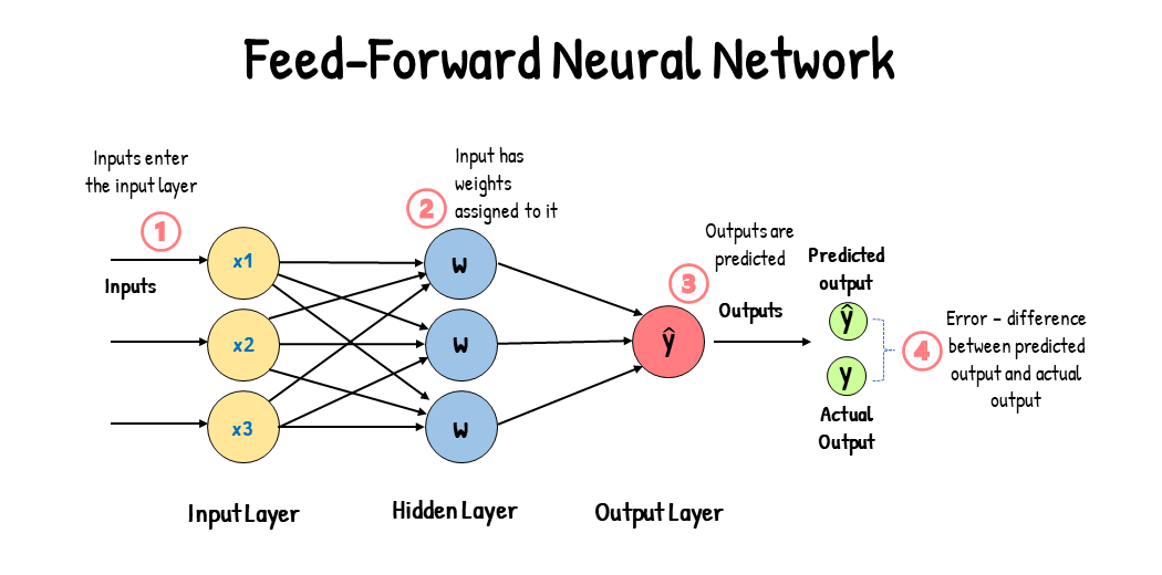
我們可以用電腦和數學運算來模擬大腦神經網路的運作
先轉換一下神經網路的模型,變成以下這樣

這裡把輸入的資料記為 $\vec{X}$,而整個神經網路中,每一條突觸 (**Synapse**) 連結都帶有一個權重 (**Weight**) $W_i$,每個神經元也都帶有偏差 (**Bias**) $b$

先計算每一組突觸連接過後的結果 $X_i \cdot W_i$ ,加上偏差 $b$,每個神經元得到結果 $z = \sum (X_i \cdot W_i) + b$

接下來,把 $z$ 帶入一個啟動函數 (**Activation Funciton**, 例如 $\sigma(z) = \frac{1}{1+e^{-z}}$ 稱為 **Sigmoid**),得到輸出訊號 $y$,再透過神經網路一層層往下傳,得到我們想要的結果。這樣就可以用電腦模擬神經元的運算了!

例如上圖,先計算 $1 \cdot 1 + (-1) \cdot (-2) + 1 = 4$,再帶入 Sigmoid 得到 $\sigma(4) = 0.98$ 作為神經元的輸出,再藉由突觸往下連接

一路計算完的結果就是這個模型的輸出

---
### Training
接下來,要訓練我們的模型,目標是**希望在給定輸入之後,可以得到期望的輸出。**
先隨機給定一些權重 $\vec{W}$ 和輸入 $\vec{X}$ ,接著透過誤差函數 (**Loss Function**) 比較輸出 ($\hat{y}$) 和正解 ($y$) 的差距 (**Loss**),最後**根據 Loss 去調整各個 Weight 和 Bias**。
調整 Weight 和 Bias 的過程稱為最佳化 (**Optimization**, 最常用的方法是梯度下降 **Gradient Descent**)。
**Gradient Descent 指的是,把誤差畫成函數圖形以後,根據斜坡的方向,朝著更低的那個點走,以此來更新 Weights**
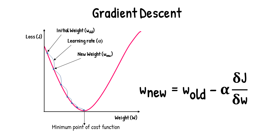
**反向傳播 (Backpropagation) 是一種加速 optimization 的過程,方法是在我得到其中一個 Weight 的 Gradient 以後透過一層層回推的方式快速反推所有其他 Weight 的 Gradient**
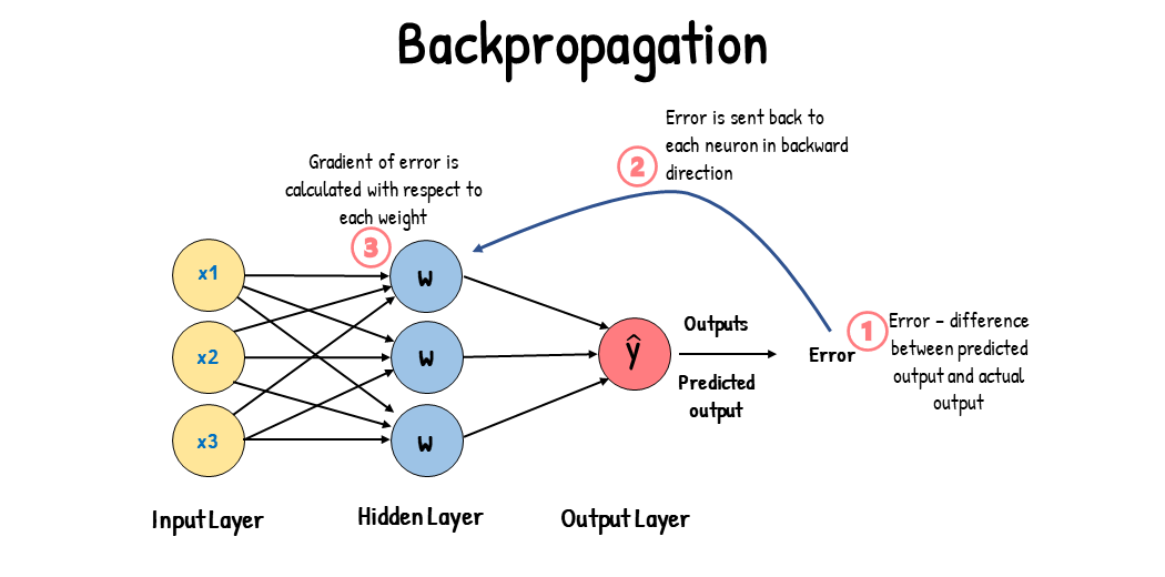
<center><small> 圖取自 analyticsvidhya.com. Gradient Descent vs. Backpropagation: What’s the Difference? </small></center>
## 實作 : MNIST 手寫辨識 (使用 Keras)
**MNIST database**(Modified National Institute of Standards and Technology database) 是來自美國國家標準技術研究所的**手寫數字資料集**
裡面包含的是 **70000 組 (60000組訓練資料 + 10000組考試資料) 圖片 (黑底白字的手寫數字) 和對應的數字**
**Keras** 是一個開源的神經網路前端,後端通常使用 tensorflow,而透過 keras 我們可以用類似拼積木的方式來建構神經網路
我們會使用這個資料集來訓練一個辨識手寫數字的 AI
**Google Colab : https://colab.research.google.com/drive/1fBz7MFxz8MJ977_qCA6zvLBw5fL3U5a2?usp=sharing**
---
安裝 **CUDA & cuDNN** (linux 可以直接用指令安裝)
CUDA: https://developer.nvidia.com/cuda/toolkit
cuDNN: https://developer.nvidia.com/cudnn
安裝相關模組 : 使用 `conda` (`miniforge`) 管理器 (推薦,可以避免許多 python 特有的怪版本問題)
```bash
conda install cudatoolkit cudnn python tensorflow-gpu keras numpy pandas matplotlib pillow scikit-learn jupyterlab
```
如果沒有 Nvidia GPU,那就不用安裝 cuda 和 cudnn,`tensorflow` 改為 `tensorflow-cpu`
---
```python=
import keras
import numpy as np
import pandas as pd
import matplotlib.pyplot as plt
```
引入相關模組
---
```python=
from keras.datasets import mnist
from keras.utils import to_categorical
# 輸入: x 輸出: y
(x_train_image, y_train_label), (x_test_image, y_test_label) = mnist.load_data()
x_trains = np.array(x_train_image).reshape(len(x_train_image), 784).astype("float64") / 255
x_tests = np.array(x_test_image).reshape(len(x_test_image), 784).astype("float64") / 255
y_trains = to_categorical(y_train_label, num_classes=10)
y_tests = to_categorical(y_test_label, num_classes=10)
```
先導入 mnist 手寫資料集
每張圖片大小是 `28*28`,所以圖集 `x` 是個三維陣列,分別是第 N 筆跟圖片的二維資料
`x.reshape` 把二維的圖片資料壓成一條一維陣列,這樣才可以對應到 784 個輸入神經元
`/ 255` 是因為每個(黑白)像素都被表示成 `0~255` 的亮度,把他轉成 `0~1` 的數值
而 `y` 代表數字資料,如果 `x[i]` 是那張圖,那麼 `y[i]` 就是數字資料
---
```python=
from keras.models import Sequential
from keras.layers import Dense, Input
layers = [
Input(shape=(784,)), # Input Layer
Dense(units=256, activation="sigmoid"), # Hidden Layer 1
Dense(units=128, activation="sigmoid"), # Hidden Layer 2
Dense(units=64, activation="sigmoid"), # Hidden Layer 3
Dense(units=10, activation="softmax"), # Output Layer
]
model = Sequential(layers)
model.summary()
```
輸入層、隱藏層、輸出層
`Sequential` 代表我們使用 $\sum x_i \cdot w_i + b$ 這樣的模型
`Dense` 代表兩兩神經元之間都有連結
分類模型的最後一層我們用 `softmax`,其他層用 `sigmoid`

---
```python=
model.compile(
optimizer=keras.optimizers.Adam(learning_rate=1e-3),
loss=keras.losses.CategoricalCrossentropy(),
metrics=[
keras.metrics.CategoricalAccuracy(),
],
)
```
建構神經網路
optimizer 使用 **Adam**
loss funcion 使用 **cross-entropy**
`metrics` 單純是 keras 如何計算誤差,不會用於訓練
---
```python=
from keras.callbacks import ModelCheckpoint, EarlyStopping
callbacks = [
EarlyStopping(patience=5, restore_best_weights=True),
ModelCheckpoint("mlp.keras", save_best_only=True)
# 某些版本要改成 mlp.tf
]
model.fit(
x=x_trains,
y=y_trains,
validation_split=0.1,
batch_size=54,
epochs=1000,
callbacks=callbacks
)
```
開始訓練模型
`callbacks` 中的 `EarlyStopping` 代表我要在模型準度沒有顯著提升後提早停止,`ModelCheckpoint` 是我把目前模型的各個參數 (Weights 和 Biases) 存下來成檔案
`validation_split=0.1` 我把 10% 的訓練資料用來計算模型的準度
`batch_size=54` 我每次觀察 54 組資料後再跑 optimization
`epoches=1000` 重複訓練 1000 次
---
```python=
from PIL import Image
fn = input("Input Filename: ")
img = Image.open(fn).resize((28, 28)).convert("L")
# Grayscale, L = R * 299/1000 + G * 587/1000 + B * 114/1000
img_proc = np.array(img).reshape(1, 784) / 255
proba = model.predict(img_proc)[0]
for cls in range(10):
print(f"{cls} with probability of {proba[cls]:.3f}")
ans = np.argmax(proba)
print("The handwritten number is:", ans)
plt.imshow(img)
```
用 `model.predict` 計算結果

---
```python=
from sklearn.metrics import confusion_matrix
y_prob = model.predict(x_tests)
y_pred = np.argmax(y_prob, axis=1)
accuracy = np.mean(y_pred == y_test_label)
print("Accuracy:", accuracy)
# Confusion matrix
cm = confusion_matrix(y_test_label, y_pred)
df_cm = pd.DataFrame(
cm,
index=[f"{i}(E)" for i in range(10)], # Expected
columns=[f"{i}(P)" for i in range(10)] # Predicted
)
df_cm
```
計算測試資料的精準度,並且作圖

---
```python=
idx = np.nonzero(y_pred != y_test_label)[0][:200]
false_pred = y_pred[idx]
false_epct = y_test_label[idx]
false_img = x_test_image[idx]
plt.figure(figsize=(14, 42))
width = 10
height = 21
for i in range(len(idx)):
plt.subplot(height, width, i+1)
t = "[E]:{}\n[P]:{}".format(false_epct[i], false_pred[i])
plt.title(t)
plt.axis("off")
plt.imshow(false_img[i])
```
列出前 200 組輸出和答案不符

---
## Appendix (Math Warning)
### Derivative & Partial
#### 微分公式 Derivative
函數 $f(x) = a_1x^n + a_2x^{n-1} + ... + a_{n-1}x^1 + a_n$ 微分後結果
$$\frac{df(x)}{dx} = (a_1 \cdot n) x^{n-1} + (a_2 \cdot (n-1))x^{n-2} + ... + (a_{n-1})x^0$$ **(次方前提次方$-1$,稱為 power rule)**
#### 偏微分 Partial Derivative
例如函數 $f(x, y) = x^2 + xy + y^2$,而 $f$ 對 $x$ 偏微代表我**只想要觀察 $x$ 的影響**,結果
$$\frac{\partial f(x, y)}{\partial x} = \frac{\partial (x^2 + yx^1 + y^2x^0)}{\partial x} = 2x + y + 0y^2 = 2x + y$$ **(Power Rule)**
#### Chain Rule
- $y = g(x) \quad z = h(y)$
$$\frac{dz}{dx} = \frac{dz}{dy} \cdot \frac{dy}{dx}$$
proof: https://math.stackexchange.com/a/1180716
- $x = g(t) \quad y = h(t) \quad z = f(x, y)$
$$\frac{dz}{dt} = \frac{\partial z}{\partial x} \cdot \frac{dx}{dt} + \frac{\partial z}{\partial y} \cdot \frac{dy}{dt}$$
proof: https://sites.und.edu/timothy.prescott/apex/web/apex.Ch13.S5.html#Thmtheorem1
圖解:
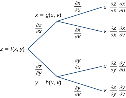
<small> 取自 math.libretexts.org. 14.5: The Chain Rule for Multivariable Functions </small>
---
### List of Activation Functions
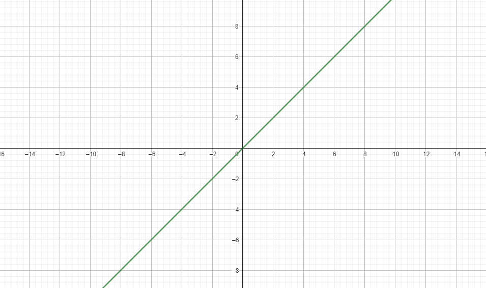
#### Indentity
$$\sigma(x) = x$$
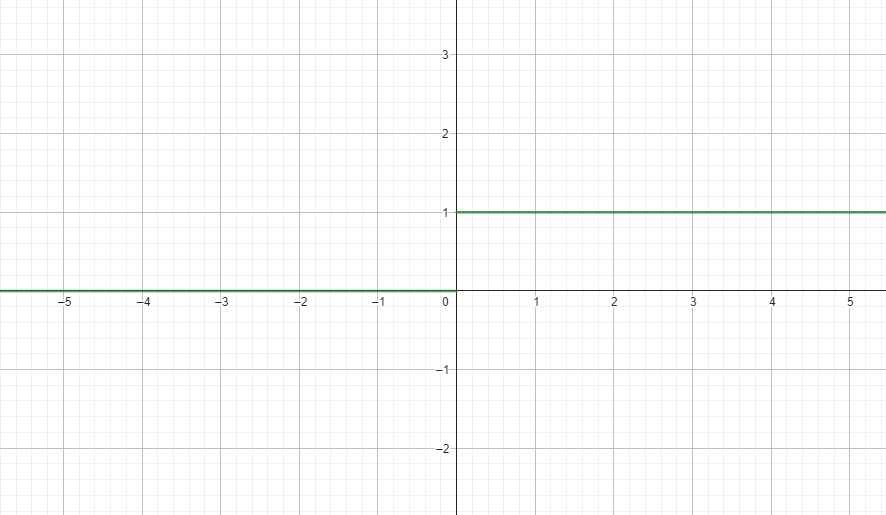
#### Binary Step / Sign
$$\sigma(x) = {\begin{cases}0&{\text{if }}x<0\\1&{\text{if }}x\geq 0\end{cases}}$$
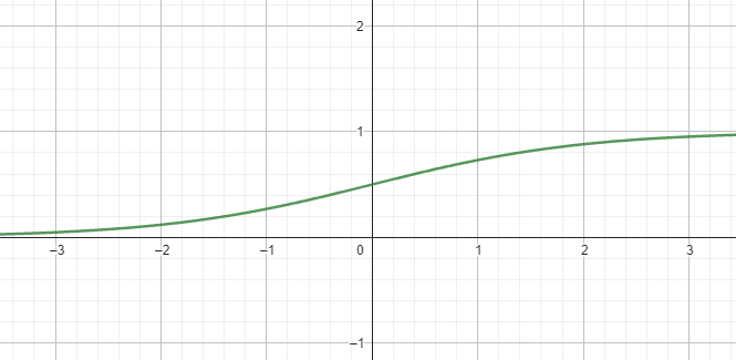
#### Sigmoid
$$\sigma(x) = \frac{1}{1+e^{-x}}$$
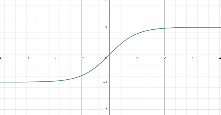
#### tanh
$$\sigma(x) = \tanh(x) = \frac{e^{x} - e^{-x}}{e^{x} + e^{-x}}$$
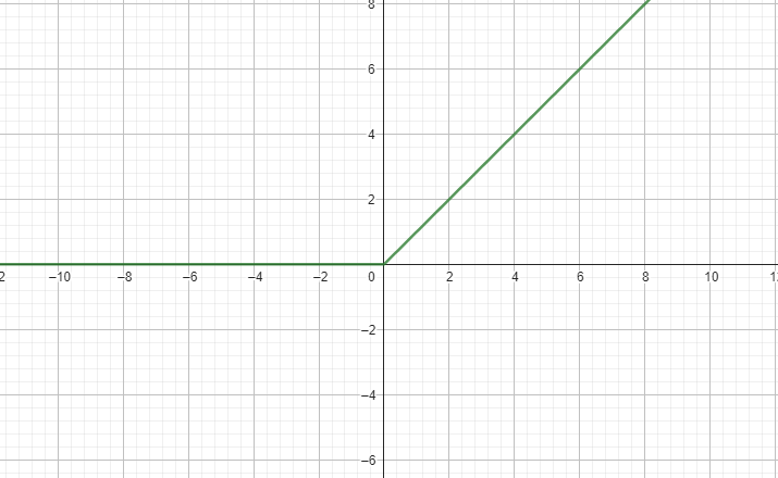
#### ReLU
$$\sigma(x) = \operatorname {max}(0, x)$$
#### Softmax
吃進一個 array 然後回傳一個 array 的 function,通常套在分類模型的 output 層之後
假設我原本有個 array $\vec{x} = (1, 4, 5, 1)$
我計算歐拉常數 $e \approx 2.718$ 的 $\vec{x}$ 次方 $e^{\vec{x}} = (2.72, 54.60, 148.41, 2.72)$
最後把每項分別除以總和 $s = \sum e^{x_i} = 208.45$
得到 $\sigma(\vec{x}) = (0.013, 0.26, 0.71, 0.013)$
寫成公式就是 $$\sigma_i(\vec{x}) = \frac{e^{x_i}}{\sum e^{x_j}}$$
套用了 softmax 後,我們的模型會畫成這樣

會用在分類型 AI 的 output layer,用處是把所有的數值轉成 0 ~ 1 的 fraction,而且總和會是 1

<center><small> 圖取自 000 機器學習簡報 </small></center>
---
### Loss Function
常見的有平均絕對值誤差 (**Mean Absolute Error**), 均方誤差 (**Mean Square Error**) 和交叉熵 (**Cross-Entropy**) 等等
#### Mean Absolute Error
$$\operatorname {MAE} = \frac{1}{N} \sum_{i=1}^N |y_i - \hat{y}_i|$$
#### Mean Square Error
$$\operatorname {MSE} = \frac{1}{N} \sum_{i=1}^N (y_i - \hat{y}_i)^2$$
#### Cross-Entropy
把模型輸出記為 $\hat{y}$, 解答記為 $y$
這裡的 $\hat{y}$ 和 $y$ 都要是機率的分布 (就是 Softmax 出來的結果)
$$\operatorname {CE} = -\sum_i \hat{y}_i \log_2 y_i$$
主要可以用在分類模型,例如以下是一個分辨動物的模型
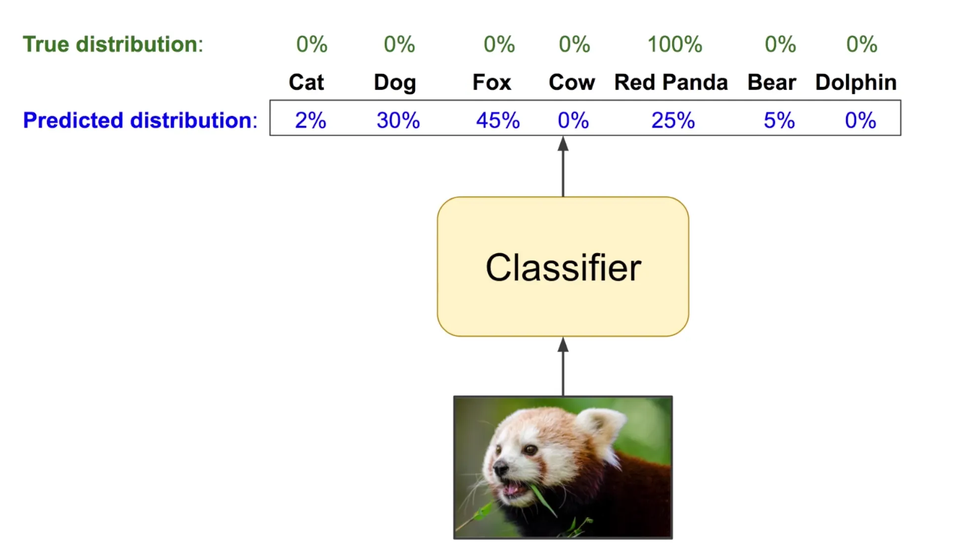
透過模型的輸出,我們可以計算 cross-entropy 作為 loss
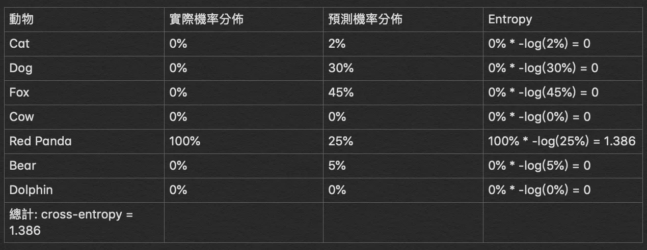
如果有一筆較精準的輸出解,cross-entropy 就會比較小
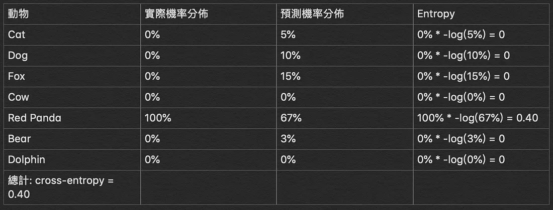
<center><small> 取自 r23456999.medium.com. 何謂 Cross-Entropy </small></center>
---
### Optimizer
#### Gradient Descent

先講梯度 (**Gradient**) 的定義
$$ \nabla f(p)={\begin{bmatrix}{\frac {\partial f}{\partial x_{1}}}(p)\\\vdots \\{\frac {\partial f}{\partial x_{n}}}(p)\end{bmatrix}}$$
而 Gradient Descent 的過程可以寫成 $$a_{t+1} = a_t - \eta \nabla f(a_t)$$ 其中 $\eta \in \mathbb {R}_{+}$ 代表學習率 (**Learning Rate**),$\eta \nabla f$ 就是我延著切線根據斜率和學習率的大小,決定 $a_{n+1}$ 要跳多少
#### Momentum
$$v_t = {\begin{cases} \eta g_t&{\text{if }}t = 0 \\ \beta v_{t-1} + \eta g_t &{\text{if }}t > 0 \end{cases}}$$
<center>
$\theta_{t+1} = \theta_t - v_t$
$g_t = \nabla f(\theta_t)$
</center>
我們把參數 (Weights and Biases) 記為 $\theta$
第一次操作就是一般的梯度下降
後面的下降速度都會加上前一個速度乘以一個阻力係數 $\beta: 0 \leq \beta < 1$
#### AdaGrad (Adaptive Gradient)
<center>
$g_t = \nabla f(\theta_t)$
$$\theta_t = \theta_{t-1} - \frac{\eta}{\sqrt{\sum_{i=1}^{t}g_i^2 + \epsilon}} \cdot g_t$$
</center>
$\epsilon$ 只是一個為了避免除以零錯誤的小數字
透過 $\sqrt{\sum_{i=1}^{t}g_i^2}$ ,我們可以做到:如果這次/前幾次 gradient 越大,學習率越小,反之則是越大,若 gradient 沒有明顯變化趨勢學習率則會慢慢變小
#### Adam
<center>
$m_t = \beta_1 \cdot m_{t-1} + (1 - \beta_1) \cdot g_{t}$
$v_t = \beta_2 \cdot m_{t-1} + (1 - \beta_1) \cdot g_{t}^2$
$\hat{m_t} = \frac{m_t}{1 - \beta_1^t} \quad \hat{v_t} = \frac{v_t}{1 - \beta_2^t}$
$$\theta_t = \theta_{t-1} - \frac{\eta}{\sqrt{\hat{v_i}} + \epsilon} \cdot \hat{m_t}$$
</center>
$\beta_1$ $\beta_2$ 是兩個介於 $[0, 1)$ 的阻尼係數
前面兩種 optimizer 的結合體,同時把 momentum 的概念套上 gradient 和 root mean square
目前使用率最高的 optimizer
他的論文 https://arxiv.org/pdf/1412.6980
---
### Backpropagation
令 loss function 為 C
$\nabla C$ 就是對於每個參數 (weights and biases) 都對 C 偏微
先觀察某個 $w$ (例如 $w_1$),目標是要算出 $\partial C / \partial w_1$
chain rule 拆解
$$\frac{\partial C}{\partial w_1} = \frac{\partial C}{\partial z} \cdot \frac{\partial z}{\partial w_1}$$

#### Forward Pass
計算 $\partial z / \partial w_1$
而 $z = x_1 w_1 + x_2 w_2 + b$
偏微結果 $= x_1$
所以 forward pass 的做法就是存前一層的輸出

#### Backward Pass
計算 $\partial C / \partial z$ 的部份比較複雜
再往下一步觀察
也就是 $\sigma(z)$,令他 $= a$
chain rule 拆成 $(\partial a / \partial z) \cdot (\partial C / \partial a )$
前項是 $\partial (\sigma(z)) / \partial z$ (Activation Function 的微分)

後項再往下拆一層
$$\frac{\partial C}{\partial a} = \frac{\partial z'}{\partial a}\frac{\partial C}{\partial z'} + \frac{\partial z''}{\partial a}\frac{\partial C}{\partial z''}$$
又 $z' = aw_3 + ...$
$\partial z' / \partial a = w_3$,同理 $\partial z'' / \partial a = w_4$
計算 $\partial C / \partial z'$

如果**下一層是輸出層**
$\partial C / \partial z'$ 是 sofmax + cross-entropy 的微分
如果不是,那麼再再繼續 chain rule 往下拆
再根據遞迴關係 (假設我已經算完 $\partial C / \partial z'$ 和 $\partial C / \partial z''$) 回來求出 $\partial C / \partial z$
backward pass 就是我從後往前 一層層推出 $\partial C / \partial z$ 的過程

#### Bias
$$\frac{\partial C}{\partial b} = \frac{\partial z}{\partial b} \frac{\partial C}{\partial z}$$
而 $z = x_1 w_1 + x_2 w_2 + b$ 可得 $\partial z / \partial b = 1$
$\partial C / \partial z$ 同上
---
### Derivative of functions
#### Sigmoid
$$\frac{d}{dx}\sigma(x) = \sigma(x)\cdot(1-\sigma(x))$$
參考 https://math.stackexchange.com/questions/78575/derivative-of-sigmoid-function-sigma-x-frac11e-x
#### Softmax + Cross-Entropy
$$\frac{\partial C}{\partial z_i} = \hat{y_i} - y_i$$
參考 https://medium.com/hoskiss-stand/backpropagation-with-softmax-cross-entropy-d60983b7b245
## References
- **000 的簡報**
https://slides.com/lucasw/machine-learning
- **000 的手刻 Neural Network**
https://github.com/lucasw0908/Neural-Network/blob/main/Neural-Network(Adam)/nn.py
- **Gradient Descent vs. Backpropagation: What’s the Difference?**
https://www.analyticsvidhya.com/blog/2023/01/gradient-descent-vs-backpropagation-whats-the-difference/
- **何謂 Cross-Entropy (交叉熵)**
https://r23456999.medium.com/%E4%BD%95%E8%AC%82-cross-entropy-%E4%BA%A4%E5%8F%89%E7%86%B5-b6d4cef9189d
- **Machine Learning 2016 Fall**
https://speech.ee.ntu.edu.tw/~hylee/ml/2016-fall.php
- **ML Lecture 3-1: Gradient Descent**
https://www.youtube.com/watch?v=yKKNr-QKz2Q&list=PLJV_el3uVTsPy9oCRY30oBPNLCo89yu49&index=7
- **ML Lecture 6: Brief Introduction of Deep Learning**
https://www.youtube.com/watch?v=Dr-WRlEFefw&list=PLJV_el3uVTsPy9oCRY30oBPNLCo89yu49&index=11
- **ML Lecture 7: Backpropagation**
https://www.youtube.com/watch?v=ibJpTrp5mcE
- **ML Lecture 8-1: “Hello world” of deep learning**
https://www.youtube.com/watch?v=Lx3l4lOrquw
## What's Next
### CNN (Covolutional Neural Network, ConvNets)
- **Breaking News, Latest News and Videos | CNN**
https://cnn.com/
- **Simple MNIST convnet**
https://keras.io/examples/vision/mnist_convnet/
- **Image classification**
https://deeplearningwithpython.io/chapters/chapter08_image-classification/
- **Convolutional Neural Networks (CNNs / ConvNets)**
https://cs231n.github.io/convolutional-networks/
### Transformer
- **Transformer: A Novel Neural Network Architecture for Language Understanding**
https://research.google/blog/transformer-a-novel-neural-network-architecture-for-language-understanding/

- **Transformer — Attention Is All You Need Easily Explained With Illustrations**
https://luv-bansal.medium.com/transformer-attention-is-all-you-need-easily-explained-with-illustrations-d38fdb06d7db
- **TRANSFORMER EXPLAINER**
https://poloclub.github.io/transformer-explainer/
- **Neural machine translation with a Transformer and Keras**
https://www.tensorflow.org/text/tutorials/transformer
- **Attention Is All You Need**
https://arxiv.org/pdf/1706.03762v7