<style>body { background-color: #eeeeee!important; } </style>
# NWO-I Software Carpentry, DIFFER 2023, day 2
:::info
:information_source: On this page you will find notes for the second day of the NWO-I Software Carpentry workshop organized on December 7
:::
<IMG SRC="https://cdn.dribbble.com/users/926537/screenshots/4502924/media/79e26abb3fb85b42f2722cf22da095dc.gif">
## Code of Conduct
Everyone who participates in Carpentries activities is required to conform to the [Code of Conduct](https://docs.carpentries.org/topic_folders/policies/code-of-conduct.html). This document also outlines how to report an incident if needed.
## :timer_clock: Schedule December 7
| | **Programming with Python**|
|------|------|
| 09:30 | Python fundamentals & analyzing tabular data |
| 10:30 | *Morning break* |
| 10:40 | Visualizing tabular data |
| 12:30 | *Lunch break* |
| 13:15 | Lists & loops |
| 15:30 | *Afternoon break* |
| 15:45 | Conditionals, functions & best practices |
| 17:30 | *END* |
## Programming with Python
### :link: Links
* Setup page: https://swcarpentry.github.io/python-novice-inflammation/index.html
* Lesson material: https://swcarpentry.github.io/python-novice-inflammation/
* Reference page: https://swcarpentry.github.io/python-novice-inflammation/reference.html
### 1. Python Fundamentals


```python!
3 * 5 + 4
weight_kg = 60
0weight_kg = 60 # invalid syntax
weight_0_kg = 60
weight_kg = 60.3
patient_id = "001"
weight_lb = 2.2 * weight_kg
patient_id = "inflam_" + patient_id
print(weight_lb)
print(patient_id)
print(patient_id, "weight in kilograms: ", weight_kg)
print(type(60.3))
print(type(patient_id))
print("weight in pounds:", 2.2 * weight_kg)
print(weight_kg)
weight_kg = 65.0
print(weight)
```

```python!
# There are 2.2 pounds in kilogram
weight_lb = 2.2 weight_kg
print("weight in kilograms: ", weight_kg, "and in pounds: ", weight_lb)
```

```python!
weight_kg = 100.0
print("weight in kilograms is now: ", weight_kg, "and in pounds: ", weight_lb)
```

:::success
:pencil: **Check Your Understanding**
What values do the variables `mass` and `age` have after each of the following statements?
Test your answer by executing the lines.
```python!
mass = 47.5
age = 122
mass = mass * 2.0
age = age - 20
```
:::spoiler :eyes: ***Solution***
```
`mass` holds a value of 47.5, `age` does not exist
`mass` still holds a value of 47.5, `age` holds a value of 122
`mass` now has a value of 95.0, `age`'s value is still 122
`mass` still has a value of 95.0, `age` now holds 102
```
:::
### 2. Analyzing Patient Data
```python!
import numpy
numpy.loadtxt(fname='inflammation-01.csv', delimiter=',')
data = numpy.loadtxt(fname='inflammation-01.csv', delimiter=',')
print(data)
print(type(data))
print(data.dtype)
print(data.shape)
print("first value in data", data [0,0])
print("middle value in data", data [29,19])
```


```python!
print(data[0:4,0:10])
print(data[5:10,0:10])
small = data[:3, 36:]
print("small is:")
print(small)
print(numpy.mean(data))
import time
print(time.ctime())
maxval, minval, stdval = numpy.amax(data), numpy.amin(data), numpy.std(data)
print('maximum inflammation:', maxval)
print('minimum inflammation:', minval)
print('standard deviation:', stdval)
patient_0 = data[0,:] # 0 on the first axis (rows), everything on the second (columns)
print('maximum inflammation for patient 0:', numpy.amax(patient_0))
print('maximum inflammation for patient 2:', numpy.amax(data[2, :]))
print(numpy.mean(data, axis=0))
print(numpy.mean(data, axis=0),shape)
print(numpy.mean(data, axis=1))
```
:::success
:pencil: **Slicing Strings**
A section of an array is called a *slice*.
We can take slices of character strings as well:
```python!
element = 'oxygen'
print('first three characters:', element[0:3])
print('last three characters:', element[3:6])
```
```
first three characters: oxy
last three characters: gen
```
What is the value of `element[:4]`?
What about `element[4:]`?
Or `element[:]`?
> :::spoiler :eyes: ***Solution***
> ```
> oxyg
> en
> oxygen
> ```
What is `element[-1]`?
What is `element[-2]`?
> :::spoiler :eyes: ***Solution***
> ```
> n
> e
> ```
Given those answers,
explain what `element[1:-1]` does.
> :::spoiler :eyes: ***Solution***
> Creates a substring from index 1 up to (not including) the final index,
> effectively removing the first and last letters from 'oxygen'
How can we rewrite the slice for getting the last three characters of `element`,
so that it works even if we assign a different string to `element`?
Test your solution with the following strings: `carpentry`, `clone`, `hi`.
> :::spoiler :eyes: ***Solution***
> ```python!
> element = 'oxygen'
> print('last three characters:', element[-3:])
> element = 'carpentry'
> print('last three characters:', element[-3:])
> element = 'clone'
> print('last three characters:', element[-3:])
> element = 'hi'
> print('last three characters:', element[-3:])
> ```
> ```
> last three characters: gen
> last three characters: try
> last three characters: one
> last three characters: hi
> ```
:::
```python!
element = 'oxygen'
element[:4]
element[-1]
element[1:-1]
```
### 3. Visualizing Tabular Data
```python!
import matplotlib.pyplot
image = matplotlib.pyplot.imshow(data)
matplotlib.pyplot.show()
ave_inflammation = numpy.mean(data, axis=0)
ave_plot = matplotlib.pyplot.plot(ave_inflammation)
matplotlib.pyplot.show()
max_plot = matplotlib.pyplot.plot(numpy.amax(data, axis=0))
matplotlib.pyplot.show()
min_plot = matplotlib.pyplot.plot(numpy.amin(data, axis=0))
matplotlib.pyplot.show()
```
```python!
import numpy
import matplotlib.pyplot
data = numpy.loadtxt(fname='inflammation-01.csv', delimiter=',')
fig = matplotlib.pyplot.figure(figsize=(10.0, 3.0))
axes1 = fig.add_subplot(1, 3, 1)
axes2 = fig.add_subplot(1, 3, 2)
axes3 = fig.add_subplot(1, 3, 3)
axes1.set_ylabel('average')
axes1.plot(numpy.mean(data, axis=0))
axes2.set_ylabel('max')
axes2.plot(numpy.amax(data, axis=0))
axes3.set_ylabel('min')
axes3.plot(numpy.amin(data, axis=0))
fig.tight_layout()
matplotlib.pyplot.savefig('inflammation.png')
matplotlib.pyplot.show()
```
:::success
:pencil: **Plot Scaling**
Why do all of our plots stop just short of the upper end of our graph?
> :::spoiler :eyes: ***Solution***
> Because matplotlib normally sets x and y axes limits to the min and max of our data
> (depending on data range)
>
> If we want to change this, we can use the `set_ylim(min, max)` method of each 'axes',
> for example:
>
> ```python!
> axes3.set_ylim(0,6)
> ```
Update your plotting code to automatically set a more appropriate scale.
(Hint: you can make use of the `max` and `min` methods to help.)
> :::spoiler :eyes: ***Solution***
> ```python!
> # One method
> axes3.set_ylabel('min')
> axes3.plot(numpy.min(data, axis=0))
> axes3.set_ylim(0,6)
> ```
> :::spoiler :eyes: ***Solution***
> ```python!
> # A more automated approach
> min_data = numpy.min(data, axis=0)
> axes3.set_ylabel('min')
> axes3.plot(min_data)
> axes3.set_ylim(numpy.min(min_data), numpy.max(min_data) * 1.1)
> ```
:::
:::success
:pencil: **Drawing Straight Lines**
In the center and right subplots above, we expect all lines to look like step functions because
non-integer value are not realistic for the minimum and maximum values. However, you can see
that the lines are not always vertical or horizontal, and in particular the step function
in the subplot on the right looks slanted. Why is this?
> :::spoiler :eyes: ***Solution***
> Because matplotlib interpolates (draws a straight line) between the points.
> One way to do avoid this is to use the Matplotlib `drawstyle` option:
>
> ```python!
> import numpy
> import matplotlib.pyplot
>
> data = numpy.loadtxt(fname='inflammation-01.csv', delimiter=',')
>
> fig = matplotlib.pyplot.figure(figsize=(10.0, 3.0))
>
> axes1 = fig.add_subplot(1, 3, 1)
> axes2 = fig.add_subplot(1, 3, 2)
> axes3 = fig.add_subplot(1, 3, 3)
>
> axes1.set_ylabel('average')
> axes1.plot(numpy.mean(data, axis=0), drawstyle='steps-mid')
>
> axes2.set_ylabel('max')
> axes2.plot(numpy.max(data, axis=0), drawstyle='steps-mid')
>
> axes3.set_ylabel('min')
> axes3.plot(numpy.min(data, axis=0), drawstyle='steps-mid')
>
> fig.tight_layout()
>
> matplotlib.pyplot.show()
> ```
> 
:::
:::success
:pencil: **Make Your Own Plot**
Create a plot showing the standard deviation (`numpy.std`)
of the inflammation data for each day across all patients.
> :::spoiler :eyes: ***Solution***
> ```python!
> std_plot = matplotlib.pyplot.plot(numpy.std(data, axis=0))
> matplotlib.pyplot.show()
> ```
:::
:::success
:pencil: **Moving Plots Around**
Modify the program to display the three plots on top of one another
instead of side by side.
:::spoiler :eyes: ***Solution***
```python!
import numpy
import matplotlib.pyplot
data = numpy.loadtxt(fname='inflammation-01.csv', delimiter=',')
# change figsize (swap width and height)
fig = matplotlib.pyplot.figure(figsize=(3.0, 10.0))
# change add_subplot (swap first two parameters)
axes1 = fig.add_subplot(3, 1, 1)
axes2 = fig.add_subplot(3, 1, 2)
axes3 = fig.add_subplot(3, 1, 3)
axes1.set_ylabel('average') axes1.plot(numpy.mean(data, axis=0))
axes2.set_ylabel('max')
axes2.plot(numpy.max(data, axis=0))
axes3.set_ylabel('min')
axes3.plot(numpy.min(data, axis=0))
fig.tight_layout()
matplotlib.pyplot.show()
```
:::
### 4. Storing Multiple Values in Lists

```python!
odds = [1, 3, 5 ,7]
print("odds are: ", odds)
print("first element" ,odds[0])
print("last element" ,odds[3])
print('"-1" element' ,odds[-1])
names = ['Curie', 'Darwing', 'Turing'] # typo in Darwin's name
print('names is originally:', names)
names[1] = "Darwin"
print('final value of names', names)
name = "Darwin"
name[0] = 'd'
mild_salsa = ['peppers', 'onions', 'cilantro', 'tomatoes']
hot_salsa = mild_salsa # <-- mild_salsa and hot_salsa point to the *same* list data in memory
hot_salsa[0] = 'hot peppers'
print('Ingredients in mild salsa:', mild_salsa)
print('Ingredients in hot salsa:', hot_salsa)
mild_salsa = ['peppers', 'onions', 'cilantro', 'tomatoes']
hot_salsa = list(mild_salsa) # <-- makes a *copy* of the list
hot_salsa[0] = 'hot peppers'
print('Ingredients in mild salsa:', mild_salsa)
print('Ingredients in hot salsa:', hot_salsa)
veg = [['lettuce', 'lettuce', 'peppers', 'zucchini'],
['lettuce', 'lettuce', 'peppers', 'zucchini'],
['lettuce', 'cilantro', 'peppers', 'zucchini']]
```
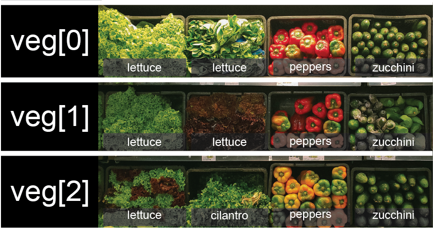
```python!
print(veg[2])
print(veg[0])
print(veg[0][0])
print(veg[1][2])
sample_ages = [10, 12.5, 'Unknown']
print(sample_ages)
print(odds)
odds.append(11)
print("odds after appending", odds)
removed_element = odds.pop(0)
print("odds after removing the first element", odds)
print("removed element:", removed_element)
odds.reverse()
print("Odds after reverse:", odds)
odds = [3, 5, 7]
primes = odds
primes.append()
print('odds:', odds)
print('primes:', primes)
odds = [3, 5, 7]
primes = list(odds)
primes.append()
print('odds:', odds)
print('primes:', primes)
binomial_name = 'Drosophila melanogaster'
group = binomial_name[0:10]
print('group:', group)
species = binomial_name[11:23]
print('species:', species)
chromosomes = ['X', 'Y', '2', '3', '4']
autosomes = chromosomes[2:5]
print('autosomes:', autosomes)
last = chromosomes[-1]
print('last:', last)
```
:::success
:pencil: **Slicing From the End**
Use slicing to access only the last four characters of a string or entries of a list.
```python!
string_for_slicing = 'Observation date: 02-Feb-2013'
list_for_slicing = [['fluorine', 'F'],
['chlorine', 'Cl'],
['bromine', 'Br'],
['iodine', 'I'],
['astatine', 'At']]
```
```
'2013'
[['chlorine', 'Cl'], ['bromine', 'Br'], ['iodine', 'I'], ['astatine', 'At']]
```
Would your solution work regardless of whether you knew beforehand
the length of the string or list
(e.g. if you wanted to apply the solution to a set of lists of different lengths)?
If not, try to change your approach to make it more robust.
Hint: Remember that indices can be negative as well as positive
> :::spoiler :eyes: ***Solution***
> Use negative indices to count elements from the end of a container (such as list or string):
>
> ```python!
> string_for_slicing[-4:]
> list_for_slicing[-4:]
> ```
:::
:::success
:pencil: **Overloading**
`+` usually means addition, but when used on strings or lists, it means "concatenate".
Given that, what do you think the multiplication operator `*` does on lists?
In particular, what will be the output of the following code?
```python!
counts = [2, 4, 6, 8, 10]
repeats = counts * 2
print(repeats)
```
1. `[2, 4, 6, 8, 10, 2, 4, 6, 8, 10]`
2. `[4, 8, 12, 16, 20]`
3. `[[2, 4, 6, 8, 10],[2, 4, 6, 8, 10]]`
4. `[2, 4, 6, 8, 10, 4, 8, 12, 16, 20]`
The technical term for this is *operator overloading*:
a single operator, like `+` or `*`,
can do different things depending on what it's applied to.
> :::spoiler :eyes: ***Solution***
>
> The multiplication operator `*` used on a list replicates elements of the list and concatenates
> them together:
>
> ```
> [2, 4, 6, 8, 10, 2, 4, 6, 8, 10]
> ```
>
> It's equivalent to:
>
> ```python!
> counts + counts
> ```
:::
### 5. Repeating Actions with Loops


```python!
odds = [1, 3, 5, 7]
print(odds[0])
print(odds[1])
print(odds[2])
print(odds[3])
odds = [1, 3, 5]
print(odds[0])
print(odds[1])
print(odds[2])
print(odds[3])
odds = [1, 3, 5, 7]
for num in odds:
print num
odds = [1, 3, 5, 7, 11, 13]
for num in odds:
print num
```
For loop in pseudo-code:
``` python!
for variable in collection:
do things
```
```python!
for x in odds:
print x
length = 0
names = ['Curie', 'Darwin', 'Turing']
for value in names:
length = length + 1
print("There are ", length, "names in the list")
name = 'Rosalind'
for name in ['Curie', 'Darwin', 'Turing']:
print(name)
print("After the loop name is:", name)
print(names)
print(len(names))
```
:::success
:pencil: **From 1 to N**
Python has a built-in function called `range` that generates a sequence of numbers. `range` can
accept 1, 2, or 3 parameters.
* If one parameter is given, `range` generates a sequence of that length,
starting at zero and incrementing by 1.
For example, `range(3)` produces the numbers `0, 1, 2`.
* If two parameters are given, `range` starts at
the first and ends just before the second, incrementing by one.
For example, `range(2, 5)` produces `2, 3, 4`.
* If `range` is given 3 parameters,
it starts at the first one, ends just before the second one, and increments by the third one.
For example, `range(3, 10, 2)` produces `3, 5, 7, 9`.
Using `range`,
write a loop that uses `range` to print the first 3 natural numbers:
```python!
1
2
3
```
> :::spoiler :eyes: ***Solution***
> ```python!
> for number in range(1, 4):
> print(number)
> ```
:::
:::success
:pencil: **Understanding the loops**
Given the following loop:
```python!
word = 'oxygen'
for char in word:
print(char)
```
How many times is the body of the loop executed?
* 3 times
* 4 times
* 5 times
* 6 times
> :::spoiler :eyes: ***Solution***
>
> The body of the loop is executed 6 times.
>
:::
:::success
:pencil: **Computing the Value of a Polynomial**
The built-in function `enumerate` takes a sequence (e.g. a [list]({{ page.root }}/04-lists/)) and
generates a new sequence of the same length. Each element of the new sequence is a pair composed
of the index (0, 1, 2,...) and the value from the original sequence:
```python!
for idx, val in enumerate(a_list):
# Do something using idx and val
```
The code above loops through `a_list`, assigning the index to `idx` and the value to `val`.
Suppose you have encoded a polynomial as a list of coefficients in
the following way: the first element is the constant term, the
second element is the coefficient of the linear term, the third is the
coefficient of the quadratic term, etc.
```python!
x = 5
coefs = [2, 4, 3]
y = coefs[0] * x**0 + coefs[1] * x**1 + coefs[2] * x**2
print(y)
```
```
97
```
Write a loop using `enumerate(coefs)` which computes the value `y` of any
polynomial, given `x` and `coefs`.
> :::spoiler :eyes: ***Solution***
> ```python!
> y = 0
> for idx, coef in enumerate(coefs):
> y = y + coef * x**idx
> ```
:::
### 6. Analyzing Data from Multiple Files

``` python!
import glob
print(glob.glob('inflammation*.csv'))
import glob
import numpy
import matplotlib.pyplot
filenames = sorted(glob.glob('inflammation*.csv'))
filenames = filenames[0:3]
for filename in filenames:
print(filename)
data = numpy.loadtxt(fname=filename, delimiter=',')
fig = matplotlib.pyplot.figure(figsize=(10.0, 3.0))
axes1 = fig.add_subplot(1, 3, 1)
axes2 = fig.add_subplot(1, 3, 2)
axes3 = fig.add_subplot(1, 3, 3)
axes1.set_ylabel('average')
axes1.plot(numpy.mean(data, axis=0))
axes2.set_ylabel('max')
axes2.plot(numpy.amax(data, axis=0))
axes3.set_ylabel('min')
axes3.plot(numpy.amin(data, axis=0))
fig.tight_layout()
matplotlib.pyplot.show()
```

:::success
:pencil: **Plotting Differences**
Plot the difference between the average inflammations reported in the first and second datasets
(stored in `inflammation-01.csv` and `inflammation-02.csv`, correspondingly),
i.e., the difference between the leftmost plots of the first two figures.
> :::spoiler :eyes: ***Solution***
> ```python!
> import glob
> import numpy
> import matplotlib.pyplot
>
> filenames = sorted(glob.glob('inflammation*.csv'))
>
> data0 = numpy.loadtxt(fname=filenames[0], delimiter=',')
> data1 = numpy.loadtxt(fname=filenames[1], delimiter=',')
>
> fig = matplotlib.pyplot.figure(figsize=(10.0, 3.0))
>
> matplotlib.pyplot.ylabel('Difference in average')
> matplotlib.pyplot.plot(numpy.mean(data0, axis=0) - numpy.mean(data1, axis=0))
>
> fig.tight_layout()
> matplotlib.pyplot.show()
> ```
:::
:::success
:pencil: **Generate Composite Statistics**
Use each of the files once to generate a dataset containing values averaged over all patients:
```python!
filenames = glob.glob('inflammation*.csv')
composite_data = numpy.zeros((60,40))
for filename in filenames:
# sum each new file's data into composite_data as it's read
#
# and then divide the composite_data by number of samples
composite_data = composite_data / len(filenames)
```
Then use pyplot to generate average, max, and min for all patients.
> :::spoiler :eyes: ***Solution***
> ```python!
> import glob
> import numpy
> import matplotlib.pyplot
>
> filenames = glob.glob('inflammation*.csv')
> composite_data = numpy.zeros((60,40))
>
> for filename in filenames:
> data = numpy.loadtxt(fname = filename, delimiter=',')
> composite_data = composite_data + data
>
> composite_data = composite_data / len(filenames)
>
> fig = matplotlib.pyplot.figure(figsize=(10.0, 3.0))
>
> axes1 = fig.add_subplot(1, 3, 1)
> axes2 = fig.add_subplot(1, 3, 2)
> axes3 = fig.add_subplot(1, 3, 3)
>
> axes1.set_ylabel('average')
> axes1.plot(numpy.mean(composite_data, axis=0))
>
> axes2.set_ylabel('max')
> axes2.plot(numpy.max(composite_data, axis=0))
>
> axes3.set_ylabel('min')
> axes3.plot(numpy.min(composite_data, axis=0))
>
> fig.tight_layout()
>
> matplotlib.pyplot.show()
> ```
:::
### 7. Making Choices

```python!
num = 37
if num > 100:
print("greater")
else:
print("not greater")
print("done")
```


```python!
num = 53
print('before conditional...')
if num > 100:
print(num, " is greater than 100")
print('...after conditional')
num = -3
if num > 0:
print(num, 'is positive')
elif num == 0:
print(num, 'is zero')
else:
print(num, 'is negative')
if (1 > 0) and (-1 >= 0):
print('both parts are true')
else:
print('at least one part is false')
if (1 < 0) or (1 >= 0):
print('at least one test is true')
```
```python!
print(data)
data = numpy.loadtxt(fname='inflammation-01.csv', delimiter=',')
max_inflammation_0 = numpy.amax(data, axis=0)[0]
max_inflammation_20 = numpy.amax(data, axis=0)[20]
if max_inflammation_0 == 0 and max_inflammation_20 == 20:
print('Suspicious looking maxima!')
elif numpy.sum(numpy.amin(data, axis=0)) == 0:
print('Minima add up to zero!')
else:
print('Seems OK!')
data = numpy.loadtxt(fname='inflammation-03.csv', delimiter=',')
max_inflammation_0 = numpy.amax(data, axis=0)[0]
max_inflammation_20 = numpy.amax(data, axis=0)[20]
if max_inflammation_0 == 0 and max_inflammation_20 == 20:
print('Suspicious looking maxima!')
elif numpy.sum(numpy.amin(data, axis=0)) == 0:
print('Minima add up to zero!')
else:
print('Seems OK!')
```
:::success
:pencil: **How Many Paths?**
Consider this code:
```python!
if 4 > 5:
print('A')
elif 4 == 5:
print('B')
elif 4 < 5:
print('C')
```
Which of the following would be printed if you were to run this code?
Why did you pick this answer?
1. A
2. B
3. C
4. B and C
> :::spoiler :eyes: ***Solution***
> C gets printed because the first two conditions, `4 > 5` and `4 == 5`, are not true,
> but `4 < 5` is true.
:::
### 8. Creating Functions

```python!
fahrenheit_val = 99
celsius_val = ((fahrenheit_val - 32) * (5/9))
print (celsius_val)
fahrenheit_val2 = 43
celsius_val2 = ((fahrenheit_val2 - 32) * (5/9))
print (celsius_val2)
def explicit_fahr_to_celsius(temp):
converted = ((temp - 32) * (5/9))
return converted
def fahr_to_celsius(temp):
return ((temp - 32) * (5/9))
```

``` python!
t1 = explicit_fahr_to_celsius(32)
print(t1)
t2 = fahr_to_celsius(32)
print(t2)
def celsius_to_kelvin(temp_c):
return temp_c + 273.15
print("the freezing point of water is ", celsius_to_kelvin(0.))
def fahr_to_kelvin(temp_f):
temp_c = fahr_to_celsius(temp_f)
temp_k = celsius_to_kelvin(temp_c)
return temp_k
print("Boiling point of water in Kelvin", fahr_to_kelvin(212.0))
print("What again is temp_k?", temp_k) # gives error, is a local variable in function
temp_kelvin = fahr_to_kelvin(212.0)
print("Temperature in Kelvin was:", temp_kelvin)
```
```python!
def visualize(filename):
data = numpy.loadtxt(fname=filename, delimiter=',')
fig = matplotlib.pyplot.figure(figsize=(10.0, 3.0))
axes1 = fig.add_subplot(1, 3, 1)
axes2 = fig.add_subplot(1, 3, 2)
axes3 = fig.add_subplot(1, 3, 3)
axes1.set_ylabel('average')
axes1.plot(numpy.mean(data, axis=0))
axes2.set_ylabel('max')
axes2.plot(numpy.amax(data, axis=0))
axes3.set_ylabel('min')
axes3.plot(numpy.amin(data, axis=0))
fig.tight_layout()
matplotlib.pyplot.show()
def detect_problems(filename):
data = numpy.loadtxt(fname=filename, delimiter=',')
if numpy.amax(data, axis=0)[0] == 0 and numpy.amax(data, axis=0)[20] == 20:
print('Suspicious looking maxima!')
elif numpy.sum(numpy.amin(data, axis=0)) == 0:
print('Minima add up to zero!')
else:
print('Seems OK!')
filenames = sorted(glob.glob('inflammation*.csv'))
for filename in filenames[0:3]:
print(filename)
vizualize(filename)
detect_problems(filename)
def offset_mean(data, target_mean_value):
return (data - numpy.mean(data)) + target_mean_value
z = numpy.zeros((2,2))
print(z)
print(offset_mean(z,3))
data = numpy.loadtxt(fname='inflammation-01.csv', delimiter=',')
print(offset_mean(data, 0))
print('original min, mean, and max are:', numpy.amin(data), numpy.mean(data), numpy.amax(data))
offset_data = offset_mean(data, 0)
print('offset min, mean, and max are:',
numpy.amin(offset_data),
numpy.mean(offset_data),
numpy.amax(offset_data))
print('std before and after', numpy.std(data), numpy.std(offset_data))
print("difference between std dev before and after", numpy.std(data)-numpy.std(offset_data))
# offset_mean will return array containing the original data with its mean offset to the desired value
def offset_mean(data, target_mean_value):
return (data - numpy.mean(data)) + target_mean_value
def offset_mean(data, target_mean_value):
"""offset_mean will return array containing the original data with its mean offset to the desired value"""
return (data - numpy.mean(data)) + target_mean_value
help(offset_mean)
numpy.loadtxt(fname='inflammation-01.csv', delimiter=',')
numpy.loadtxt('inflammation-01.csv', delimiter=',')
numpy.loadtxt('inflammation-01.csv', ',')
def offset_mean(data, target_mean_value=0.0):
return (data - numpy.mean(data)) + target_mean_value
test_data = numpy.zeros((2,2))
print(offset_mean(test_data, 3))
more_data = 5 + numpy.zeros((2,2))
print("data before mean offset:")
print(more_data)
print("offset data:")
print(offset_mean(more_data))
def display(a=1, b=2, c=3):
print('a ', a, 'b ', b, 'c', c)
print("no parameters")
display()
print("one parameter")
display(55)
print("two parameters")
display(66)
print("only setting one parameter")
display(c=77)
```
:::success
:pencil: **Return versus print**
Note that `return` and `print` are not interchangeable.
`print` is a Python function that *prints* data to the screen.
It enables us, *users*, see the data.
`return` statement, on the other hand, makes data visible to the program.
Let's have a look at the following function:
```python!
def add(a, b):
print(a + b)
```
**Question**: What will we see if we execute the following commands?
```python!
A = add(7, 3)
print(A)
```
> :::spoiler :eyes: ***Solution***
> Python will first execute the function `add` with `a = 7` and `b = 3`,
> and, therefore, print `10`. However, because function `add` does not have a
> line that starts with `return` (no `return` "statement"), it will, by default, return
> nothing which, in Python world, is called `None`. Therefore, `A` will be assigned to `None`
> and the last line (`print(A)`) will print `None`. As a result, we will see:
> ```
> 10
> None
> ```
:::
```python!
help(numpy.loadtxt)
```

### 9. Errors and Exceptions

```python!
# This code has an intentional error. You can type it directly or
# use it for reference to understand the error message below.
def favorite_ice_cream():
ice_creams = [
'chocolate',
'vanilla',
'strawberry'
]
print(ice_creams[3])
favorite_ice_cream()
def some_function()
msg = 'hello world!'
return(msg)
print(a)
letters = ['a', 'b', 'c']
print('Letter #1 is', letters[0])
print('Letter #5 is', letters[5])
file_handle = open('myfile.txt', 'r')
```
 Sign in with Wallet
Connect another wallet
Sign in with Wallet
Connect another wallet