# Computorv2 & Computorv1
This note will be focused on the things I have learnt while doing the 2 computor projects in 42. This will mostly be on computorv2 since its an extension of the first one and its is more complex.

Both of the projects require us to receive an equation as an input and we are required to evaluate the equation and display the result(s) as the output. Something like a mini-calculator.

[ToC]

## Evaluation

> [comptutation](https://www.mathsisfun.com/definitions/computation.html)

Before we get into the computation of any mathemathical equation, we would have to evaluate it first so that we know what should be computed, in what order.

Suppose our input is something simple, like `1 + 2 + 3 = ?`, its pretty straightforward that we need to first compute `1 + 2`, then use the result and compute `result + 3` to ge the final answer.

The expression above is considered in a _normal form_ because it cannot be reduced even further. expressions like `1 + x + f(y)` can still be reduced further, given that x is a variable with a value and f(y) is a function that returns a value with `y` as the object.

There are 2 widely used strategies to reduce any expression to its normal form
- Normal order evaluation
- Reduces and evaluates from left to right
- Applicative order evaluation
- Reduces and evaluates from inner most function to outer most function

Heres an example where we have 2 functions,

def double(x): 
   return x + x

def avg(lhs, rhs):
    return (lhs + rhs) / 2

and our expression to evaluate is

double(avg(2, 4))

Reducing this using the **Normal order evaluation** will result in steps taken below:

double(avg(2, 4))
avg(2, 4) + avg(2, 4)
(4 + 2) / 2 +  avg(2, 4) # normal form is detected!!
3 + avg(2, 4)
3 + (4 + 2) / 2 # normal form is detected!!
3 + 3
6

Reducing this using the **Applicative order evaluation** will result in steps taken below:

double(avg(2, 4))
double((4 + 2) / 2) # normal form is detected!!
double(3)
3 + 3  # normal form is detected!!
6

Notice how the `avg()` function got called twice and how we are passing unevaluated functions in the normal order evaluation. Though this might looks like a small difference since the output is the same, there are actually cases where it will generate different output for each strategy.

Consider we have the following function added

def cond(condition, valA, valB):
    if condition is True:
        return valA,
    return valB

the function above will return `valA` if the `condition` is `True` or `valB` otherwise.

We will try to evaluate the following function:
`cond(True, 69, 420)`

**Normal order evaluation**

cond(True, double(1), sqrt(-1))
if True return double(1) else sqrt(-1)
if True return 1 else sqrt(-1) # normal form detected!!
1

**Applicative order evaluation**

cond(True, double(1), sqrt(-1))
if True return 1 + 1 else √-1 # error
Error, √-1

Notice that Applicative order evaluation throws an error because it tried to compute `sqrt(-1)` which is impossible. However Normal order evaluation ignores that computation because `if True return 1` already satistied its evaluation requirements and proceeds with the computation

## Parse tree generation

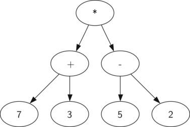
Above is a parse tree generated by the mathematical equation `((7 + 3) * (5 - 2))`. A parse tree is used so that smaller components can be isolated inside the subtrees and can be resolved independently. The tree can only be generated once there equation is grouped correctly and its fully parenthesised(?).

:::warning
:bulb: **Warning:** `1 + 2 + 3 + 4` isnt valid to generate a parse tree, it needs to be converted to `((1 + 2) + (3 + 4))` first. We'll discuss on the conversion part in the later section.
:::

Of course, at this point we are assuming that our expression is already broken down to a bunch of tokens, e.g. `['(', '3', '+', '(', '4', '*', '5' ,')',')']` and each token is already labelled with a type for identification.

> We know that '(' is a parenthesis, '5' is a number, '/' is an operator and so on...

To generate a parse tree, we would go through every token in our token list and execute the operations based on the rules below.

1. If the current token is a `(`, add a new node as the left child of the current node, and descend to the left child.
2. If the current token is in the list `['+','-','/','*']`, set the root value of the current node to the operator represented by the current token. Add a new node as the right child of the current node and descend to the right child.
3. If the current token is a number, set the root value of the current node to the number and return to the parent.
4. If the current token is a `)`, go to the parent of the current node.

Below is an example of the steps taken to generate the parae tree for expression `['(', '3', '+', '(', '4', '*', '5' ,')',')']`.









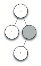
Step by step desciprtions:
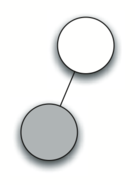
1. Create an empty tree.
2. Read ( as the first token. By rule 1, create a new node as the left child of the root. Make the current node this new child.
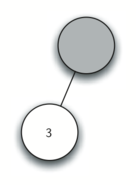
3. Read 3 as the next token. By rule 3, set the root value of the current node to 3 and go back up the tree to the parent.
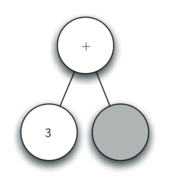
4. Read + as the next token. By rule 2, set the root value of the current node to + and add a new node as the right child. The new right child becomes the current node.
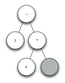
5. Read a ( as the next token. By rule 1, create a new node as the left child of the current node. The new left child becomes the current node.
6. Read a 4 as the next token. By rule 3, set the value of the current node to 4. Make the parent of 4 the current node.
7. Read * as the next token. By rule 2, set the root value of the current node to * and create a new right child. The new right child becomes the current node.
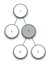
8. Read 5 as the next token. By rule 3, set the root value of the current node to 5. Make the parent of 5 the current node.
9. Read ) as the next token. By rule 4 we make the parent of * the current node.
10. Read ) as the next token. By rule 4 we make the parent of + the current node. At this point there is no parent for + so we are done.
## Parse tree computation
To compute a generated parse tree, we start from the lowest subtree which only has an operator node and 2 operant children, substitute the operator node with the result of the computation using the 3 terms from the nodes above, and repeat this process on the next lowest subtree until the root of the tree is substituted.

The procedure will look like this is code:
1. If current node is a child or null, return
2. Traverse left child (recurse)
3. Traverse right child (recurse)
4. If current node has only 1 children, replace current node with child and return
5. If current node has 2 leaf children, evaluate and subsitute curr node

Below is an example of steps taken to compute the parse tree above:

1. Starts at the root node, traverses left child
2. current node does not have children, return to root which will then traverse right child
3. There are 2 leaf children at current node
4. Compute `(4 * 5)` and replace the result at current node
5. Right traverse returns to root node, there are 2 leaf children at current node
6. Compute `(20 + 3)` and replace the result at current node

The result of the entire expression is stored in the root node.

## Token preprocessing
As we see earlier, we are only able to generate a parse tree and compute said parse tree iff we have correctly formatted expressions (correct grouping and parentheses). We will be discussing about pattern grouping and preprocessing in this section.

But first, we need to decide what is our goal and desired format to acheive. A term can be a number, float, matrix or any representation of a value. Any terms can be joined together using operators `(+, -, *, /, ...)`. For instance, `41` is a term, `12 + 12` are 2 terms joined by a `+`. A group is a number terms wrapped in parentheses `()` and can be joined together using operators like terms. `(1 + 2 + 3 - 1)` is a group of 4 terms, `((1 + 2) + (3 - 2))` is a group of 2 groups.

Since our tree is a binary tree, in order to make the rules for parse tree generation to give us the tree we wants, our end tokens needs to :
- have at most 2 terms / groups (operand operator operand).
- have at most 2 terms / groups inside each parentheses.
- pair and group terms with a maximum of 2 terms per group in the event of the current scope exceeding 2 terms.

Below are some examples of tokens before and after preprocessing:

1 + 2 + 3 + 4 + 5
((1 + 2) + (3 + 4)) + 5

1 + 2 + 3 + 4 
(1 + 2) + (3 + 4)

1 + 2 + (3 + 4) + 5
((1 + 2) + ((3 + 4))) + 5

1 + (2 + (3 + 4)) + 5
(1 + (2 + (3 + 4))) + 5

There are many ways to fill in the extra parentheses, but a loop with a few counters should do ;)

:::info
:bulb: **Hint:** To comply with the BODMAS rules, we need to encapsulate the terms surrounding a priority operator `{*, /, ^}` so that they will appear lower in the parse tree and will get evaluated first.
:::

## Theorems and algorithms
### Euclidean algorithm for GCD resolution
>[wiki](https://en.wikipedia.org/wiki/Euclidean_algorithm#CITEREFStark1978)

Like the title suggests, the Euclidean algorithm is an algorithm to find the Greatest Common Divider (GCD) of 2 whole positve numbers. This is required to simplify fractions to its most simplest form for `computorv1` bonus.

The algorithm suggests that:
$$
a = q_{1}b + r_{0}\\
b = q_{2}r_{0} + r_{1}\\
r_{0} = q_{3}r_{1} + r_{2}\\
r_{1} = q_{4}r_{2} + r_{3}\\
..\\
..\\
r_{n - 4} = q_{n - 2}r_{n-3} + r_{n-2}\\
r_{n - 3} = q_{n - 1}r_{n-2} + r_{n-1}\\
r_{n - 2} = q_{n}r_{n-1} + 0\\
$$
Where $r_{n - 1}$ is the GCD of $a$ and $b$ Hence, it encapsulates into the procedure
$$
GCD(a, b) = GCD(b, a\mod b)
$$

Quite straightforward, but how does it work?
First, we need to establish some axioms, and our proofs will be based on these axioms

Axiom #1:
$$
\forall a \in \mathbb{N} .\ GCD(a, 0) = a
$$
> For all natural numbers `a`, the GCD of that number with 0 will be equals to `a`

Axiom #2:
> This recursive function will eventually end, since this pattern of modulo will eventually reach zero.

With that in mind, the following will prove that $r_{n - 1}$ is indeed a common divisor of $a$ and $b$.

$$
r_{n - 1} | \ a \\
r_{n - 1} | \ b
$$

_Proof:_
The last line of the sequence
$$
..\\
r_{n - 2} = q_{n}r_{n-1} + 0\\
$$
Showed us that $r_{n-1}$ divides $r_{n - 2}$. If thats the case, then the line previously $r_{n - 3} = q_{n - 1}r_{n-2} + r_{n-1}$, $q_{n - 1}r_{n-2} + r_{n-1}$ can be expanded to $(r_{n-2} + r_{n-2} \ ... \ q_{n - 1} \ times + r_{n-1} + r_{n-1}\ ...\ q_{n} \ times)$. Which shows us that $r_{n-1}$ also divides $r_{n-3}$.

This cascading will carry on until the top 2 sequences where $r_{n-1}$ divides both $a$ and $b$. _qed_

Which will then be used to prove
$$
GCD(a, b) = GCD(b, a\mod b)
$$

will eventually end with

$$
GCD(x, 0)
$$

Where `x` is the `GCD` of `a` and `b`
_Proof:_
Suppose that we have a number $d$ that has the property $d |a$ and $d|b$($d$ divides $a$ and $d$ divides $b$). If $d$ has such a property, then $d$ should divide $a - bq_{1}$ which is equals to $r_{1}$.

For such a number that divdes $r_{1}$, that number should also divide $r_{2}$ based on the proof above. With this conclusion, we know that this sequence of numbers will eventually lead to $d$ being able to be divide $r_{n-1}$ which is the GCD of $a$ and $b$.

If the number exists, then
$$
GCD(a, b) = GCD(b, a\mod b)
$$
would hold true, and the GCD of $a$ and $b$ will be $r_{n - 1}$ when
$$
GCD(r_{n - 1}, 0)
$$
### Newton's method for square root resolution
> [wiki](https://en.wikipedia.org/wiki/Newton%27s_method)

A naive way of determining a square root of a number is to iterate through all possible positive integers and test them one by one by squaring them and compare the result of the number we want to test, stopping the iteration when the squares of the current iteration is more than the number we want to test.

This will work to a certain extent on perfect squares, but even so, if the number we want to test isnt a perfect square, we wont be able to get decimal precise answers and this process will have a growth factor of $O(n)$ where $n$ is the range between 1 to the square root of the input.

There is an algorithm that will resolve this for us, the idea is that we make an initial guess on what the square root of a number is, then we will compare our guess with the actual result by dividing the target number with our guess and we can determine if our guess hits the spot given a tolerance range. If it doesnt, we improve our guess and the algorithm goes through another iteration.

The procedure goes like this :
$$
x_n = x_{n-1} - \frac{f(x_n))}{f'(x_n))}
$$

Where $x_n$ is the new approximation, $x_{n-1}$ is the previous or initial approximation and $f$ is the function to approximate the roots of.

If we want to evaluate sqaure root of 2, our $f$ can be defined as $f(x) = x^2 - 2$, and our derivative, $f'(x) = 2x$

We can start the procedure by having initial guess, 1
$$
x_1 = 1 - \frac{f(1))}{f'(1))} \\
x_1 = 1.5
$$

We then check that $x_1$ does indeed equal to itself when divided by 2.
$$
2 / x_1 = 1.333\\
1.333 \neq x_1
$$

Looks like its false, we will do another iteration again

$$
x_2 = 1.5 - \frac{f(1.5))}{f'(1.5))} \\
x_2 = 1.416
$$
$$
2 / x_2 = 1.416\\
1.412 \neq x_2
$$
Looking at how this is going, we will eventually reach converge to a point where $x_n \approx 2/x_n$, then we can say that $x_n$ will be our square root.

How does it work?
Suppose we plot $f(x)$ to a graph:

We can tell that the gradient of tangent at point $(x_n, f(x_n))$ is equal to $f'(x_n)$ and $\frac{f(x_n) - 0}{x_n - x_{n + 1}}$

Since $x_{n + 1}$ is our next approximation, we can substitude the equation above to obtain $x_{n - 1}$ into
$$
x_{n + 1} = x_n - \frac{f(x_n)}{f'(x_n)}
$$
thus validating the algorithm.
### Evaluating trigonometric functions using the Taylor series
> [wiki](https://en.wikipedia.org/wiki/Taylor_series)

To compute the trigonometric functions without using a refrence table , $sin(30) = 0.5$, $sin(90) = 1$ ... , we can utilize the taylor series and the [Trigonometric derivatives](https://en.wikipedia.org/wiki/Differentiation_of_trigonometric_functions) to generate a close approximation of a trigonometric function for us with any input.

The Taylor series or Taylor expansion of a function is an infinite sum of terms that are expressed in terms of the function's derivatives at a single point.

:::info
:bulb: **Hint:** In more simple terms, the Taylor series is a polynomial that approximates the rate of change of a graph around a single point.
:::

A typical taylor series is described like so:
$$
f(a) + \frac{f^{'}(a)}{1!}(x - a)^1 + \frac{f^{''}(a)}{2!}(x - a)^2 + \frac{f^{'''}(a)}{3!}(x - a)^3+...
$$
Which can be simplified to :
$$
\sum_{n = 0}^{\infty }\frac{f^{n}(a)}{n!}(x - a)^n
$$
where $f^{n}(a)$ denotes the nth derivative of $f$ evaluated at the point $a$. (The derivative of order zero of $f$ is defined to be $f$ itself and $(x − a)0$ and $0!$ are both defined to be 1.)

To calculate the value of any trigonometric function using Taylor series, we will define $a = 0$. and we replace the function $f$ with the trigonometric function that we want to evaluate.

For sin(x):
$$
sin(x) = sin(0) + \frac{sin^{'}(0)}{1!}x^1 + \frac{sin^{''}(0)}{2!}x^2 + \frac{sin^{'''}(0)}{3!}x^3+...
$$

$$
sin(x) = 0 + \frac{cos(0)}{1!}x^1 + \frac{-sin(0)}{2!}x^2 + \frac{-cos(0)}{3!}x^3+...
$$

$$
sin(x) = 0 + \frac{1}{1!}x^1 + \frac{0}{2!}x^2 + \frac{-1}{3!}x^3+...
$$

$$
sin(x) = \frac{x}{1!} - \frac{x^3}{3!}+...
$$

$$
\sum_{n = 0}^{\infty }\frac{(-1)^n}{(2n+1))!}(x)^{2n+1}
$$

### Matrix inversion using Minors, Cofactors and Adjugate
>https://www.mathsisfun.com/algebra/matrix-inverse-minors-cofactors-adjugate.html

## Design pattern
>[Composite design pattern](https://en.wikipedia.org/wiki/Composite_pattern)

>In software engineering, the composite pattern is a partitioning design pattern. The composite pattern describes a group of objects that are treated the same way as a single instance of the same type of object.

The subject requires us to be flexible between number types, as in we are allowed to do operations on different number representations as if they are the same. Instead of having 4 handlers for all types of numbers, I encapsulated all the number types into a `BaseAssignmentType` and made my function to do operations on `BaseAssignmentType`s alone.

My `Matrix`, `RationalNumber`, `ImaginaryNumber` and `Function` all inherits from `BaseAssignementType` and is able to be type casted to their native types when needed.


###### tags: `algo` `math` `computorv2`