---
tags: carpentry
robots: noindex, nofollow
---
# CHC DC Workshop notes: Day 2
* This Hack MD: http://bit.ly/chc_dc_notes_day2
* Zipped data files https://csuchico.box.com/s/inbszas47mnx0apjrxai88562sx4xopt
****
# 09:00-09:15 Recap
* Thank you for sticky note feedback
* revised the lesson today
* sent out a glossary /recap of yesterday's important vocabulary with links to "cheatsheets"
* Hack MD
* cleaned up
* Split into day 2 since no external helpers
* collaborative! You get to keep these notes later. Put your own notes in here.
* navigation bar
## What we covered
* Spreadsheets to store data
* saved in a common format
* comma separated values (`.csv`) or tab separated (`.txt` or `.tsv`)
* raw data never touched
* Good ML vs Bad ML
* tidy data priciples -- (one observation per row, one column per variable)
* better collection == less cleanup
* Goal is reproducibility
* Effort up front for payoff in time later
* scripting is the only way to ensure reproducibility
* Open Refine is a great tool for text cleaning
* spreadsheet like interface
* it has options for validating and converting data types (number, date etc)
* creates a script that can be applied at a later point
* undo/redo capabilities
* requires java, can stick/hang during download.
* don't forget to _extract_ the zip file before you try to run
* R vs R Markdown vs R Studio
* R is the programming Language (the engine)
* R Studio is the bright orange pt cruiser convertable that we get to drive R around in
* R Markdown allows us to combine english with R code to make literate documents
* Using Packages: what are they, installing, using
* Assigning data to objects using `<-` (called assignment operator)
* Data/Object types
* integer/numeric, character/factor, dates/times, boolean (new; statement that is TRUE/FALSE)
* can be identified using `str`, `class`, and `typeof` functions in R.
* Object types: `vector` (one collection of numbers or characters) vs `data.frame` (collection of numbers or characters) vs `table` (ex: frequency table to summarize data) vs `tibble` (spreadsheet like but has some extra functionalities)
* Be explicit when describing what you need - there are different terminologies depending on who you are talking too.
* Example Final Products
* Pretty PDF report for external audience
* C:\Box\Projects_Current\Chemistry Redesign\Spring18 updates\code
* Expoloratory survey analysis
* C:\Box\CHEM Studio\code\fac_staff
* Daily process and progress reports (health check)
* C:\Box\CHC - CalFresh Outreach Program Reporting - Level 1\scripts
## What we're going to cover today
* How to get help
* Help panel
* In RStudio go to Help –> Cheatsheets
* Communities: RUG, DSI
* Your neighbor
* Navigating data frames
* How to identify specific rows and columns
* Advanced data management and aggregation with `dplyr`
* Making pretty pictures with `ggplot`
* looking forward
## Some helpful set-up commands
* tools --> globaloptions
* uncheck `Restore .RData into workspace at startup`
* `Save workspace to .Rdata on exit` click the drop down and select never
# 09:15-10:00 Exploring the SAFI data
* set global options (see instructions above)
* restart R studio
#### Exercise #1
1. Create a new R markdown file. (Ctrl + Alt + I)
2. Clear out all the template language below the first code chunk
3. Re-read in the `SAFI_Clean` data into an object called `interviews`
* **Don't reinvent the wheel! Go find the code from yesterday and copy that into the first code chunk**
* Click the green play button to run this single code chunk interactively (live)
4. In a new code chunk display the first 6 rows of the data by typing `head(interviews)`
* run this code chunk by clicking the green play button
This is often referred to as _"Calling head on interviews"_.
> Point out how executing a code chunk copies the code from the script window down into the console. You can turn off it displaying in the script window and just have it display in the console and vice versa - it is what you prefer.
>
> Demo <kbd>CTRL</kbd>+<kbd>ENTER</kbd>
Data Frame == columns of vectors of different data types

#### Exercise 1b. Get Esther's helper code
If you haven't done so yet, download the zipped files for this workshop from the link at the top of this page and unzip into your workshop folder.
Open the `Summary of terms.Rmd` file by double clicking --> Knit.
**Indexing**
* uses brackets: [rows, columns]
What does the first row/col look like?
> point out word wrapping with tibble output
> Call `head()` on the fifth column.
#### Exercise #2. Average number of years living in the village
1. Click the blue arrow to the left of the `interviews` data frame in the *environment* to see the list of variable names.
2. What column is the variable `years_liv` in?
3. Using bracket notation, and the `mean()` function, what is the average number of years a farmer has been living in their village?
What if you had hundreds of variables? How would you find the column number?
* you don't. You call the variable by its variable name instead using `$` notation.
> general format `data$variable`
This is Base R code. It's a tried and true standard way of calling variables by name.
_We'll see something slightly different with dplyr_
#### Exercise #3. Frequency tables
Using `$` notation, and the `table()` function, create a frequency table for the `village` variable. _(i.e.,call `table()` on `interviews$village`)_
****
# 11:00-11:30 Data management with `dplyr`

* Reminder about what packages are
* install `dplyr`
* Explain why `dplyr` is better suited for some data management tasks than what we saw on day 1
* consistent grammer. data set name is always first
* explain / list (write on board?) 7 common functions (verbs) that we're going to cover
1. `select` - gets columns
2. `filter`- gets rows
3. `mutate` - make new columns (variables)
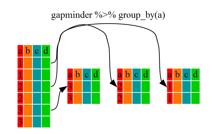
4. `group_by` goes with
5. `summarise` - create aggregated statistics
6. `count` - tabulate (count number of rows..)
Selecting columns and filtering rows
`select` columns 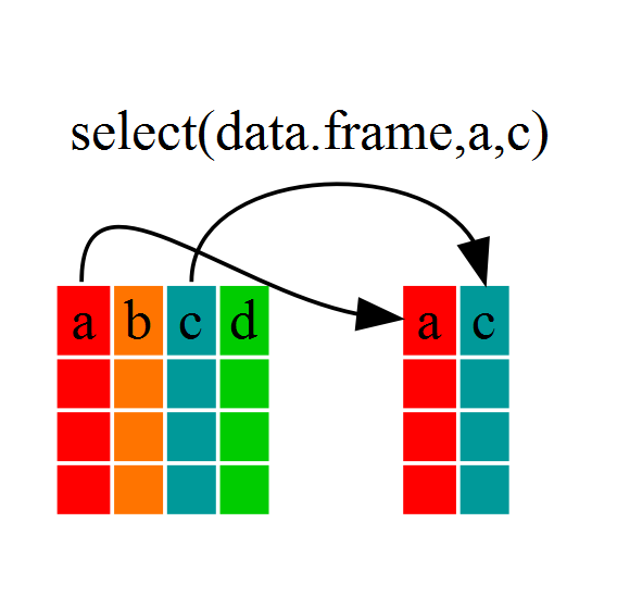
* select `village` and `interview date`
* You can view, or save as a new data frame
* No $ sign is needed here.
Note: Selecting is useful for narrowing your purpose (variables you want to look at specifically)
"Cannont find function" error --> forgot to load package
##### Exercise #1. Make a new data frame with four variables: `affect_conflicts`, `liv_count`, and `no_meals` and `village`. Name this new data frame `safi_conflict`
```{r}
safi_conflict <- select(interviews, affect_conflicts, liv_count, no_meals, village)
```
`filter` rows (subsetting/just like Excel's filter)
* uses logical statements
* shows rows where the statement is TRUE
* ==, >, <, <=, >=
* they live alone `filter(interviews, no_membrs<1)`
* save as new data set
* call `dim()` on new data to see count
* look in environment to get count
* alternative statement no_membrs==0
##### Exercise #2. Filter the `safi_conflict` data to only include farmers from the village God. Save this as a new data frame called `god_conflict`.
**Solution:** `god_conflict<-filter(safi_conflict, village == 'God')`
Multiple statements using & and |
`filter(interviews, no_membrs>5 & rooms<2)`
`filter(interviews, no_membrs==1 | village=="God")`
Pipes `%>%` chain commands together
> "Put the thing on the left of the pipe, in the first argument in the statement on the right."
Read `%>%` as "And Then"
```{r}
interviews %>% select(no_membrs, village, rooms)
```
Take the interviews data set, and then...
selct these columns
```{r}
interviews %>%
select(no_membrs, village, rooms) %>%
filter(rooms<2)
```
*Shortcut-* `ctrl+shift+M` adds pipe for you without having to type `%>%`
#### Exercise #3: Combine the steps in exercise 1 and 2 into a single line. I.e. start with `interview`, end with `god_conflict`, bypassing `safi_conflict`.
---
**LUNCH**
----
`mutate` makes new columns.
* interviews %>% mutate(people_per_room = no_membrs / rooms)
#### Exercise #2: Create a new data frame (`meals_gt_20`) from the interviews data that meets the following criteria:
* contains only the village column and a new column called `total_meals` containing a value that is equal to the total number of meals served in the household per day on average (`no_membrs*no_meals`).
* Only the rows where `total_meals` is greater than 20 should be shown in the final data frame.
_Hint: think about how the commands should be ordered to produce this data frame!_
* start with interviews
* select varibles no_members, no_meals, village (optional here)
* create new variable total_meals as no_membrs*no_meals
* filter total_meals < 20
* select total_meals and village
1. create new data frame called `meals_gt_20`
2. start with interviews
3. select varibles no_members, no_meals
4. create new variable total_meals as no_membrs*no_meals
5. filter total_meals > 20
```{r}
meals_gt_20 <- interviews %>%
mutate(total_meals=no_membrs*no_meals) %>%
filter(total_meals > 20) %>%
select(village, total_meals)
meals_gt_20
```
## Split-apply-combine data analysis and the summarize() function
`group_by`
`summarize`
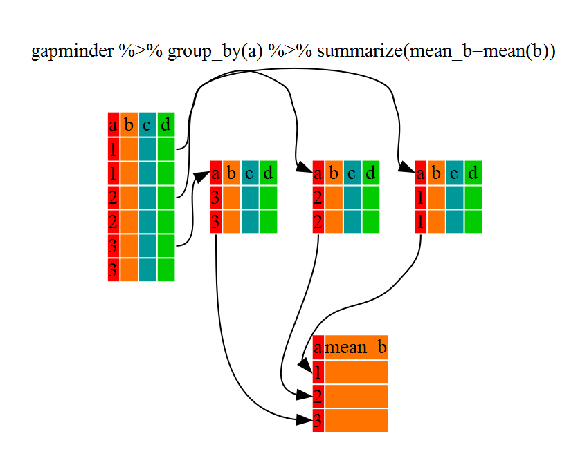
* Compute the average household size by village:
`interviews %>%
group_by(village) %>%
summarize(mean_no_membrs = mean(no_membrs))`
* summarize is like mutate in that it creates a new variable, but NOT like mutate in that it is a summary number (one number is created per group)
* nested groups
`interviews %>%
group_by(village, memb_assoc) %>%
summarize(mean_no_membrs = mean(no_membrs))`
### Counting
* interviews %>% count(village)
vs
* table(interviews$village)
Same information is presented
* using `count` presents the data as a data.frame, not as a table. This will let us plot this summary information later.
#### Exercise #3: Create summary measures
1. How many households in the survey have an average of two meals per day?
2. Three meals per day?
3. Are there any other numbers of meals represented?
*skip*
****
# Data Visualization
* package name `ggplot2`
* function name `ggplot`
* general structure of code
`ggplot(data, aes(x=x, y=y)) + geom_THING()`
2.1.1 Required arguments
data: What data set is this plot using? This is ALWAYS the first argument.
aes(): This is the aestetics of the plot. What’s variable is on the x, what is on the y? Do you want to color by another variable, perhaps fill some box by the value of another variable, or group by a variable.
geom_THING(): Every plot has to have a geometry. What is the shape of the thing you want to plot? Do you want to plot points - use geom_points(). Want to connect those points with a line? Use geom_lines(). We will see many varieties in this lab.
* categorical vs continuous (numeric)
* village = category
* no_membrs = continuous
* barplot village
`ggplot(interviews, aes(x=village)) + geom_bar()`
* histogram no_members (boxplot, density)
* no_membrs
* no_members by village -- to add grouping by a categorical variable, use `fill` or `color`inside the `aes()` argument
* scatterplot: no_membrs vs years_liv
* add line
* col village
* facet on village instead
* facet_grid
the point is that it's a small amount of code can make a big plot.
## references
* https://norcalbiostat.github.io/AppliedStatistics_notes/the-syntax-of-ggplot.html
* http://www.cookbook-r.com/Graphs/
# 14:00 - 14:30 ML work
* Open refine combined_log_raw --> combined_ml_clean
* Walk through analysis in `ml_viz`
> Show State demog code
* emphasize that the data owner needs to see your work
* ran report before cleaning (assumed people entered in 'x's correctly)
# 14:45 Showcase, brainstorm, open work
* [Blog/project aware Websites](http://www.norcalbiostat.com/)
* [Static websites](https://norcalbiostat.github.io/MATH615/)
* Nicely formatted tables
* [Lecture Notes](https://norcalbiostat.github.io/AppliedStatistics_notes/index.html)
* [Books / guides](https://bookdown.org/yihui/bookdown/)
* Presentations https://rpubs.com/sdplus/vulcan74
* Dashboards
* [sales report](https://beta.rstudioconnect.com/jjallaire/htmlwidgets-highcharter/htmlwidgets-highcharter.html#sales-by-category)
* [dynamic views](https://bookdown.org/csgillespie/shiny_components/#htmlwidget-and-value-boxes)
* [storyboards](https://beta.rstudioconnect.com/jjallaire/htmlwidgets-showcase-storyboard/htmlwidgets-showcase-storyboard.html)
* ["live streaming"](https://gallery.shinyapps.io/cran-gauge/)
* [Interactive maps](https://shiny.rstudio.com/gallery/superzip-example.html) --> **JANESSA!!!!**
* [animation]()
16:00 Wrap-up
16:30 Post-workshop Survey
 Sign in with Wallet
Connect another wallet
Sign in with Wallet
Connect another wallet