# 15/6

- Learning through Tensorflow’s TFAgents library: https://www.tensorflow.org/agents/overview

## Policy Gradient Methods

Sub-class of Policy-Based Methods which estimate an optimal policy's weights through **gradient ascent**

- Stochastic or deterministic policy:

For stochastic, neural network output an action vector representing a probability distribution.

- Key idea for policy gradients:

Reinforce good actions!

Push up probabilities of actions leading to higher return, push down probabilities of actions leading to lower return -> until optimal policy

## REINFORCE

### 1. Trajectory

State-Action-Reward sequence, no restriction in length, can be a full or part of an episode -> search optimal policy for both **episodic** and **continuous** tasks.

$$\tau = (s_0, a_0, r_1, s_1, a_1, r_2, s_2, ..., a_H, r_{H+1}, s_{H+1})$$

### 2. Return of a trajectory

$R(\tau)$ is sum of reward of trajectory $\tau$

$$R(\tau) = (G_0, G_1, ..., G_H)$$

where $G_k$ is total return (or future return) at time step $k$ for transition $k$

$$(s_k, a_k, r_{k+1})$$

which is return we expect to collect from time step $k$ until end of trajectory

# Current work

## 1. First Attempt

### State Representation:

array([[3, 0],
       [5, 0],
       [1, 0],
       [4, 3],
       [5, 0],
       [5, 0]])

array([3, 0, 5, 0, 1, 0, 4, 3, 5, 0, 5, 0])

where for example `[3, 0]` means row `1` has `3` containers and `0` overstow.

### Action representation:

Discrete(30)

> convert_action_to_log(13) # convert action 13 to moving container

    Moving container from row 3 to row 5

where each action is mapped to moving a container from `row_origin` to `row_dest`

### Implementation of Environment:

[OpenAI Gym](https://github.com/openai/gym)

### Code

- Actor-Critic Algorithm:

https://colab.research.google.com/drive/1xE_Ik2Wyda20TWX7pt0uvAm-jwunzZyN?usp=sharing

## 2. Second Attempt

### State Representation:

array([[[1, 1, 1],
        [1, 1, 1],
        [1, 1, 0],
        [0, 0, 0],
        [0, 0, 0],
        [0, 0, 0]],

       [[1, 1, 0],
        [1, 1, 0],
        [1, 1, 0],
        [1, 1, 0],
        [0, 0, 0],
        [0, 0, 0]],

       [[1, 1, 0],
        [1, 1, 0],
        [1, 1, 0],
        [0, 0, 0],
        [0, 0, 0],
        [0, 0, 0]],

       [[1, 0, 1],
        [1, 0, 1],
        [1, 0, 0],
        [0, 0, 0],
        [0, 0, 0],
        [0, 0, 0]],

       [[1, 0, 0],
        [1, 0, 0],
        [0, 0, 0],
        [0, 0, 0],
        [0, 0, 0],
        [0, 0, 0]],

       [[1, 1, 0],
        [1, 1, 0],
        [1, 1, 0],
        [1, 1, 0],
        [0, 0, 0],
        [0, 0, 0]]], dtype=int32)

This array is of shape `(6, 6, 3)`.

For example, `[[1, 1, 1],
[1, 1, 1],
[1, 1, 0],
[0, 0, 0],
[0, 0, 0],
[0, 0, 0]]` indicates the current state of a row `1`. Each entry represent a container level. Index `0` of container level `[1, 1, 1]` indicates a container is present. Indexes `1` and `2` for `[1, 1, 1]` indicates overstowed and mixPSCW respectively.

### Code

- Actor-Critic

https://colab.research.google.com/drive/1Mh5V2lBKrDth-9iEx_PsIeWJxliHGM0h?usp=sharing

- Deep Q-Network

https://colab.research.google.com/drive/1Ubgs0PTK9IYNveO02qlZ_cXlsEZo_T4t?usp=sharing

# Difficulties

- Unable to extract actions that lead to the current state after training.

Suspected to be due to:
#### 1. Poor state representation
#### 2. Poor reward distribution
#### 3. Too many actions

- Currently:

Enhancing the state and modifying reward.

# 17/6

## Successes

- In simple cases where there are only 1 or 2 moves away from the goal state, the agent can reach it with different possibilities.

## Learning points

- It is very important for the agent to reach terminal state for each episode in order to train effectively.

- Previously, the terminal state is when all rows have no overstow but sometimes during training the agent seldom or never reaches this state to learn effectively -> terminating state is relaxed then can work for simple case

- Parameter tuning is so very important:

1. Episode length: currently set up 100 to ensure the agent can reach terminal state. Must be taken in consideration with goal reward such that agent will not try to go circular to maximise episode reward which exceeds terminating at goal.

2. Terminating reward threshold:

- This threshold needs to be set properly as well in order to make sure the model can accurately predict best action at a given state.

## Thoughts

- Need to come up with some metrics to determine appropriate reward, cost depending on how many containers are currently in block, how many free spaces and ground slots

- For instance, based on that computation, what is the maximum episode reward achievable? What will be the terminal state? That will determine how much final state is rewarded as well.

- Now kinda able to get the solution, but need to encode negative reward for each move too, so as to minimise the number of moves.

- Consider greedy: freeze those rows already correct, don't move them around but only place container on top of them.

- Also, restrict the action space if possible, so that convergence during training is more likely.

## Implementation plans

For tomorrow:

- Implement action space restriction with ground slots consideration

- Try out current implementation on both overstow and mix weight

- Try out current implementation on slot with 3 moves away from optimal

For the weekend:

- Study this repository https://github.com/giladariel/Connect4 for sample implementation of tic tac toe (see state, reward, episode parameters)

- Study tensorflow in depth https://www.tensorflow.org/tutorials/images/transfer_learning

# 18/6

- Experiment with both overstow and mix weight

# 21/6

- Try out Sudoku Monte Carlo Tree Search from this repository https://github.com/int8/monte-carlo-tree-search

- Rewrite the reward function

- Use Deep Q-Network for now, will try Double Deep Q-Network (actor-critic) from TF-Agents

- Currently, ground slot is negatively rewarded and agent has avoided touching it

# 22/6

## Thoughts

- Overstow should be heavily penalised with higher cost

- Different vessel if overstow will incur additional cost

- Different vessel with no overstow will still be okay

- Similarly for different port mark and category they will only be penalised if there's overstow

- Weight is only considered given same vessel, same port mark, same category

## Implementations

- Implement cost computation for vessel, port mark, category and weight

- Could generate desirable actions if terminating condition is not too strict (overall cost is <= 2 instead of 0)

- Prepare powerpoint slides for meeting tomorrow

https://docs.google.com/presentation/d/1M2R-sVkb-y2AUzxRPQFLH6AsOQA3vwyxfK8roUF1V6o/edit?usp=sharing

## To do

- Implement for size as well

- Test and fine-tune for different scenarios, conduct comparative studies for hyperparameter tuning

- Try out a combination with MTCS as a heuristic so that better actions are tried out first

# 23/6

## Implementation

- Include all elements for now

## Successes

- If terminal state is set as having the cost reduced by half or more, the DQN successfully suggests a number of good movements

## Discussion with HoD

- Reminders: consider stochastic elements in reality as well (changing portmarks or etb) since etb is just expected time

- It's possible to move containers across slots in reality

- Have to consider whether RL can train across a number of examples and then generalize to a model that can handle new circumstances

## Further research

- Mixed Integer Programming

- RL applied in MIP by DeepMind

- Explore metaheuristic algorithms such as greedy randomized adaptive search procedure (GRASP) in combinatorial optimization problems.

# 24/6

## Readings Summary

---

### DQN:

https://storage.googleapis.com/deepmind-media/dqn/DQNNaturePaper.pdf


---

### Branch and Bound Algorithm

https://www.youtube.com/watch?v=gGQ-vAmdAOI&t=26s&ab_channel=MITOpenCourseWare

- A* algorithm: Combination of both extended list + branch and bound + admissible $H(x, G) \leq D(x, G)$ and consistent heuristic $H(x_1, G) + H(x_2, G) \leq D(x_1, x_2)$

https://www.youtube.com/watch?v=R6BQ3gBrfjQ&list=PLTZbNwgO5eboLWN702BfpEvPShGjjlZgr&index=2&ab_channel=saurabhschool

- For Knapsack Problem: Can formulate it into a MIP problem too with **Maximization and Constraint**


- Maintain sum of benefits so far + sum of weights so far + upper bound of benefits for each node

- Extend breadth-wise until a solution is achieved (goal state)

- Maintain a **global highest benefits** achieved by **all solutions so far**

- Use Fractional Knapsack sum of benefits as upper bound for each state. Greedily explore node with highest upper bound first.

- Update global benefits if goal state reached

- Prune away nodes where their upper bound is lower than global benefits


### Solving MIP with Neural Network

https://arxiv.org/pdf/2012.13349.pdf

### Stochastic Gradient Descent:

https://blog.paperspace.com/intro-to-optimization-in-deep-learning-gradient-descent/

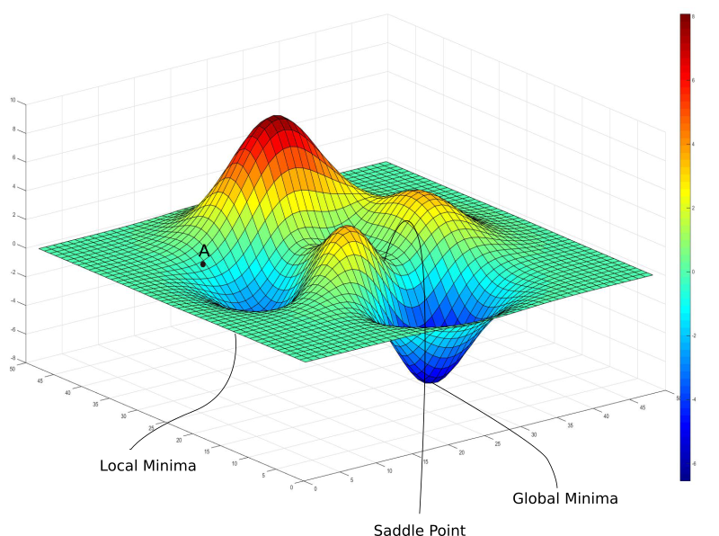
- Local minima and saddle points


- Learning rate decay (simulated annealing (heat treatment to enhance durability of material))

- Batch vs stochastic and mini-batch gradient descent (randomness)

### Heuristics for optima search based on past behavior of gradient:

https://blog.paperspace.com/intro-to-optimization-momentum-rmsprop-adam/

#### Pathological (physical or mental illness) curvation:

Where learning rate has decayed thus moves very slowly but may not be in the direction of the weights that reduce the loss most -> false impression of convergence


#### Gradient descent is First Order Optimization Method:

Where it is only aware of direction of the loss (whether it is decreasing) and how fast, but not the curvation of loss function -> Second Order Derivative to know how quickly **the gradient itself is changing**

#### Newton's Method:

Computing Hessian Matrix (a matrix of double derivatives of loss function w.r.t all combinations of weights) can give ideal step size to move in direction of gradient but it's huge and costly


---

#### Momentum:

- Instead of using only the gradient of the current step to guide the search, momentum also accumulates the gradient of the past steps to determine the direction to go.



We are taking an exponential average of the gradient steps.


Each gradient update has been resolved into components along w1 and w2 directions. If we will individually sum these vectors up, their components along the direction w1 cancel out, while the component along the w2 direction is reinforced.

---

#### RMSProp (Root Mean Square Propogation):

- No need to adjust learning rate by doing it automatically by choosing a different learning rate for **each parameter**.


First equation compute exponential average of square of gradient. Since we do it separately for each parameter, gradient Gt here corresponds to the projection, or component of the gradient along the direction represented by the parameter we are updating.

Notice our diagram denoting pathological curvature, the components of the gradients along w1 are much larger than the ones along w2. Since we are squaring and adding them, they don't cancel out, and the exponential average is large for w2 updates.

---

#### Adam (Adaptive Moment Optimization):

- RMSProp and Momentum take contrasting approaches. While **momentum accelerates our search in direction of minima, RMSProp impedes our search in direction of oscillations.** Adam combines both above heuristics.


We compute the exponential average of the gradient as well as the squares of the gradient for each parameters (Eq 1, and Eq 2). To decide our learning step, we multiply our learning rate by average of the gradient (as was the case with momentum) and divide it by the root mean square of the exponential average of square of gradients (as was the case with momentum) in equation 3. Then, we add the update.

### Vanishing Gradients and Activation Function

https://blog.paperspace.com/vanishing-gradients-activation-function/

- Neural networks make no probabilistic or statistical assumptions about the data fed.

- But a key element is that data fed to layers of NN exhibit these properties

#### Properties:

1. Data distribution **zero centered**. Absence of this can cause **vanishing gradients**

2. Distribution preferrably **normal**. Absence of this can cause **overfit**

3. Distribution of the activations should remain constant as training goes. Absence of this is called **Internal Covariate shift**

---

#### Vanishing Gradients


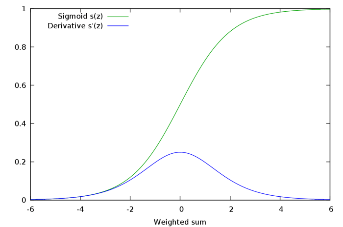
Problem with Sigmoid at very small or large end -> gradient near zero

- Gradients of deeper neurons vanish due to chain rule which contains gradient of sigmoid activation which is between 0 and 1 so when many of them are multiplied -> overall product times 0 -> so learning doesn't take place.

- Saturated Neurons: when $w^Tx + b$ either very high or low is fed into a neuron with Sigmoid action so gradient of sigmoid is nearly 0 -> no update to $w$ and $b$

---

#### ReLU

- The product of gradients of ReLU function doesn't end up converging to 0 as the value is either 0 or 1. If the value is 1, the gradient is back propagated as it is. If it is 0, then no gradient is backpropagated from that point backwards

- One-sided Saturations:

In contrast to two-sided saturations in sigmoid.

Serve a purpose that when input to ReLU becomes more and more negative, we just output 0 as a switch off.

We'd like to think neurons in a deep network like switches, which specialize in detecting certain features, which are often termed as concepts.

Neurons in the higher layers specialize in detecting high level concepts like eyes, tyres. Neurons in lower layers specialize in low-level concepts such as curves, edges.

We want neurons to fire when such concept is present in input and magnitude is maintained as a measure of **extent of that concept**. However, for negative input values, it is more convenient (otherwise would be hard to interpret) to just assign 0 to signify **absence of concept**.

- Information Disentanglement and Robustness to Noise: As variance produced in the positive output of neuron is fine as we want magnitude as an indicator of strength of signal but undesirable variance due to noise produced in negative output is avoided.

- Sparsity: Makes network train faster as computation of activation is much simpler than sigmoid and when negative preactivations is set to zero this produces sparsity to be exploited for computational benefits.

---

#### Dying ReLU Problem

- Too much sparsity hamper learning: If the weights and bias learned is such that the preactivation is negative for the entire domain of inputs, the neuron never learns, causing a sigmoid-like saturation.

- Zero-centered activations: ReLU only output non-negative activations

Hence, Sign of gradient update for all neurons is the same, all weights in a layer $l_n$ can either increase or decrease during one update.

This produces a zig zag pattern in search of minima which slows down training.


---

#### Leaky ReLUs and Parameterized ReLUs


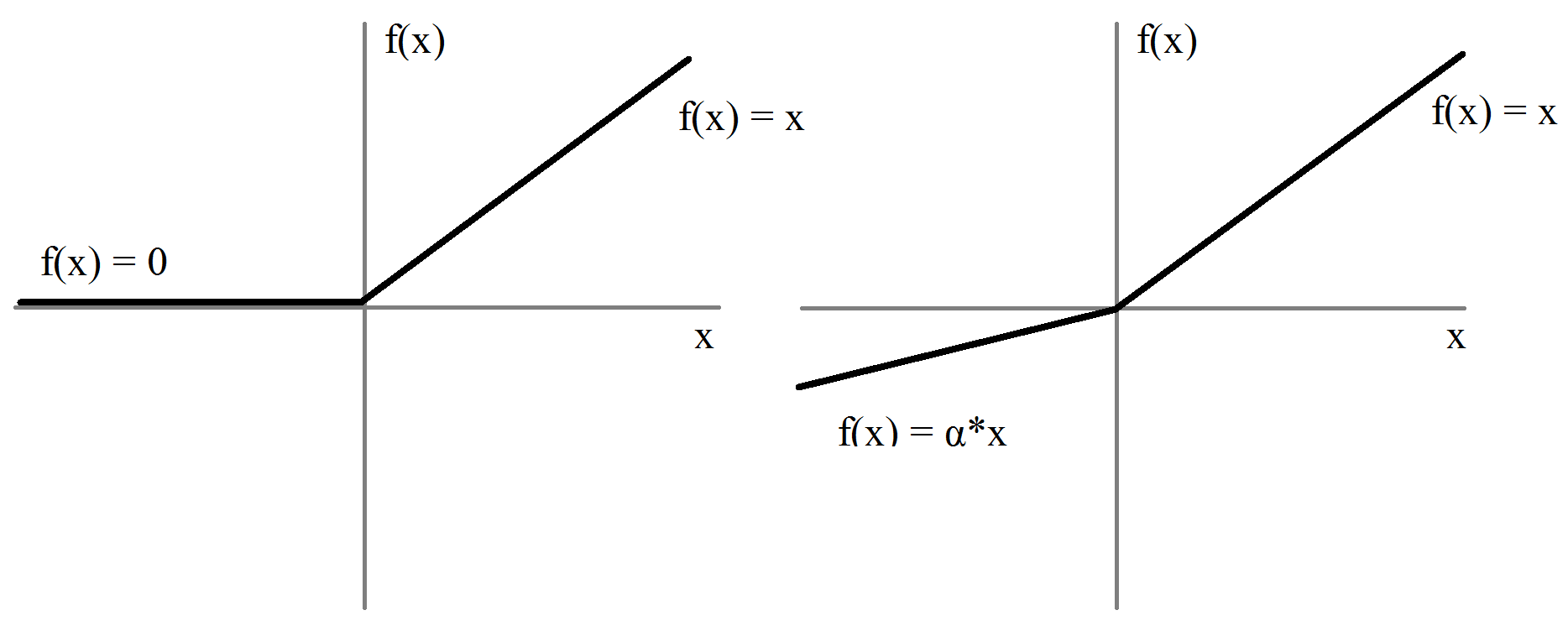
- Combat dying ReLUs: when $x < 0$, some negative slope is allowed.

Weights can now be updated in both directions.

- Considerations for randomizing $\alpha$ to stay away from local minima and saddle points

---

#### Parameterized ReLUs

- Instead of randomly sampling negative slope $\alpha$, turn it into a hyperparameter to be learned by the network during training.

---

#### Exponential Linear Units and Bias Shift

Perfect activation function has two desirable properties

1. Producing a zero-centered distribution, which can make the training faster.

2. Having one-sided saturation which leads to better convergence.

While Leaky ReLUs and PReLU solve the first condition, they fall short on the second one. On the other hand, a vanilla ReLU satisfies the second but not the first condition.

An activation function that satisfies both the conditions is an Exponential Linear Unit (ELU).


$$
f(x)=
\begin{cases}
x,& \text{when } x > 0\\
\alpha(e^x - 1), & \text{when } x \leq 0
\end{cases}
$$

Since $e^x \to 0$ as $x \to -\infty$

### Batch Normalization

https://blog.paperspace.com/busting-the-myths-about-batch-normalization/

Need for a constant and well behaved distribution of data being fed to layers of a neural network for it learn properly.

While activation functions implicitly try to normalize these distributions, a technique called Batch Normalization does this explicitly

1. Zero-centered

2. Constant through time and data: distribution of the data being fed to the layers should not vary too much across the mini-batches fed to the network, as well it should stay somewhat constant as the training goes on.

---

#### Internal Covariate Shift


So during backward pass, distribution of output of layer c denoted as $z_c$ changes, hence learning for layer d is affected.

---

#### Batch Normalisation


Equations 2-3 calculates mean and variance of each activation across a mini-batch. Equation 4 normalize to mean zero and standard deviation 1. Equation 5 is the magic that transform output of the layer to mean $\beta$ and standard deviation $\gamma$.

---

#### Why does Batch Norm work?

- Deep Neural networks have higher-order interactions, which means changing weights of one layer might also effect the statistics of other layers in addition to the loss function. These cross layer interactions, when unaccounted lead to internal covariate shift. Every time we update the weights of a layer, there is a chance that it effects the statistics of a layer further in the neural network in an unfavorable way.

- Batch Normalization does not solve ICS. However, when we add the batch normalized layer between the layers, the statistics of a layer are only effected by the two hyperparameters $\gamma$ and $\beta$.

- Now our optimization algorithm has to adjust only two hyperparameters to control the statistics of any layer, rather than the entire weights in the previous layer. This greatly speeds up convergence, and avoids the need for careful initialization and hyperparameter tuning.

- Batch Norm also acts as a regularizer: The mean and the variance estimated for each batch is a noisier version of the true mean, and this injects randomness in our optima search. This helps in regularization.

# 25/6

## Readings

---

### Bipartite Graphs

https://en.wikipedia.org/wiki/Bipartite_graph#:~:text=In%20the%20mathematical%20field%20of,the%20parts%20of%20the%20graph


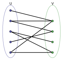
- Can be divided into 2 sets of nodes such that each edge connect 2 nodes one from each set.

- Equivalent to: graph is 2-colorable and there is no odd cycle

## Topics to explore

### Graph Theory

### RL Algorithms

---

#### Double Q-learning

https://arxiv.org/abs/1509.06461

- RL is about learning good policies to solve sequential decision problems by optimizing a cumulative future reward. However, even with DQN, there's a problem of overestimation of action values.

- To solve sequential problems, we learn some estimates for the optimal value of each action, defined as the expected sum of future rewards when taking that action and following the optimal policy thereafter.



- DQN signatures:

1. Target Network: Using parameter $\theta^-$. Target network copies parameters from online network every $\tau$ steps so that $\theta^- = \theta$ for the next steps. This is to stablize the target for training. Otherwise, it would get updated at every step because this target is an approximation dependent on the parameters $\theta$ itself!

New target is thus:


2. Experience Relay: Observed transitions are stored for some time and sampled uniformly from memory bank to update the network. This leads to greater efficiency of past data as well as decorrelating consecutive samples.

- For both equations $2 \text{ and } 3$, the max operator uses the same values both to select and evaluate an action. This makes it more likely to select overestimated values. So value estimations is overoptimistic -> decouple selection from evaluation

- Double Q-learning: Two value functions are learned by assigning each experience randomly and update one of two value functions such that there are two set of weights, $\theta$ and $\theta'$. For each update, one set of weights is used to determine the greedy policy and the other determine its value. So we can untangle the selection and evaluation in Q-learning to rewrite 2 targets:



- Double DQN: Reduce overestimations by decomposing the max operation in the target into action selection and action evaluation. So online network is used to evaluate greedy policy while the existing target network is used to estimate value. Below is the new value estimate using weights $\theta^-$


---
#### AlphaGo Zero

https://www.nature.com/articles/nature24270

https://web.stanford.edu/~surag/posts/alphazero.html

> 2 main components:

1. Neural Network: Input is current state $s$, 2 outputs

- A continuous value of the board state $v_\theta(s) \in [-1, 1]$ as the reward prediction of this state. Actual reward is either 1 or -1

- A policy $\vec{p}_\theta(s_t)$ which is probability vector over all possible actions

Loss is a combination of mean square error and cross entropy


Underlying idea: Over time, the network will learn what states eventually lead to wins (or losses). Meanwhile, learning the policy would give a good estimate of what the best action is from a given state.

2. Monte Carlo Tree Search for Policy Improvement:

Given state $s$, neural network provides an estimate of policy $\vec{p}_\theta$. During training, we want to improve these estimates.

We will expand the search tree gradually, one node at a time.


- Initialize empty search tree with $s$ as root

- A single simulation is as followed:

* Compute action $a$ that maximises upper confidence bound $U(s, a)$

* If next state $s'$ obtained from $s, a$ exists in tree, recursively call search on $s'$. Else, add new state to tree and initialise $P(s', .) = \vec{p}_\theta(s')$ and $v(s') = v_\theta(s')$ from neural network and initialize $Q(s', a)$ and $N(s', a)$ to 0 for all $a$. Instead of performing rollout, popagate $v(s')$ along path seen in current simulation and update all $Q(s, a)$ values. Otherwise, if we encounter a terminal state we propagate the actual reward back.

* After a few simulations, $N(s, a)$ values at root provide a better approximation for the policy. Improved stochastic policy $\vec{\pi}(s)$ is just the normalized counts $N(s,.)/\sum_b(N(s,b))$. During self-play, we perform MCTS and pick a move by sampling a move from improved policy $\vec{\pi}(s)$

> Policy Iteration through Self-Play

1. Initialize neural network with random weights, starting with a random policy and value network

2.

---

#### Monte-Carlo Tree Search

https://www.youtube.com/watch?v=vDF1BYWhqL8&t=968s&ab_channel=stanfordonline

### MIP and Linear Programming

---

#### Convex Set

- If S is a convex set and $x_1, x_2, ..., x_k$ are any points in it, then X is also in S where X is:

$$X = \sum^k_{i=1}\lambda_ix_i\text{ where} \lambda_i > 0 \text{ and} \sum^k_{i=1}\lambda_i = 1$$

Which means that S is a convex set when some linear combinations of some points in S with sum of coefficients equals 1 will produce a point also in S.


---

#### Solve a Linear Programming problem with Graphical Method


- Only for 2 variables optimisation problem due to complexity of visualization. For each constraint, draw a line representation, check which side is the satisfying side. After all constraints, we get a region of feasible solutions.

- To find optimal solution from this region, draw the objective function with some initial value, then depending on max or min optimisation, move in the direction until the corner of the region (by convex theorem it is the optimal solution)

- Some LP problem is not feasible

---

#### Elementary Row Operations (EROs)


- Similar to matrix operations in solving system of linear equations

---

#### Simplex Method to solve LP



---

#### Solve Linear System of Equations using Gauss Jordan Method


- Special cases: No solution or infinite number of solutions

---

#### Basic and Non-basic variables

- Simplex method: Standardize problem by adding slack variables $S_i$



---

#### Integer LP using Branch and Bound


- Simplex and other methods cannot work when it is a MIP (variables are integer) problem. Use Branch and Bound

- First relax integer condition to get an upper bound

- Also, the feasible solutions are only integer points inside the original yellow region

- Start with an upper bound using relaxed condition and variable values

- For each branching node, it is a subproblem with additional constraints, which can be inputted in some solver


- Actually in the above example, can stop after first node branched out because $Z = 27$ which is the best we can get given relaxed upper bound being $27.67$

### Graph Neural Network (Graph Convolutional Network)

http://web.stanford.edu/class/cs224w/

---

#### Why Graphs?

- Many natural phenomenon has a graph-like relationship underneath, so being able to learning this representation is the goal

- Neural network has been traditionally tuned to work with linear representation (fixed size as well as simple topology such as left-right, down-up) but we want to input graph structure instead which is unfixed


- GCN is used in DeepMind paper

---

#### Applications of Graph ML


---

#### Choice of Graph Representation

- Similar to graph theory

---

#### Traditional Feature-based Methods: Node

# 28/6

## Operations Research

https://towardsdatascience.com/what-is-operations-research-1541fb6f4963

- Linear Programming

- Queuing Theory

- Inventory Control Systems

- Replacement Problems

- Network Analysis

- Sequencing Problems (our problem)

## Readings

---

### Learning Combinatorial Optimization Problems over Graphs

https://papers.nips.cc/paper/2017/file/d9896106ca98d3d05b8cbdf4fd8b13a1-Paper.pdf


## Linear Programming continue

### Big M Method

- When there are constraints with $\geq$ or $=$ signs

- Excess and artificial variables: first 3 equations we can add slack variables cus it's $\leq$, but fourth equation we have to use excess $e_4$ and artificial $a_4$ to make it equals. $a_4$ will be added to objective function with a very large coefficient so we hope to maximize objective function, we will reduce value of $a_4$ to 0


### Dual Programming

---

#### - Relationship between Primal and Dual LP



#### - Write dual programming of a primal LP program



### Dual Simplex Method


- 2 conditions need to be satisfied before Dual Simplex

1. Objective function must satisfy optimality condition: if it's a min problem, all coefficients must be positive and vice versa

2. We have at least one constraint with $\geq$ or $=$ sign


### Transportation problem


- Supply must be $\geq$ to demand

- 3 methods to find a feasible solution

---

#### Northwest Corner


- Doesn't take transportation cost into account so will be likely less optimal

---

#### Minimum Cost


---

#### Vogel's Method


---

#### Unbalanced Case where Supply > Demand


### Optimize a Transportation Problem



### Solve an assignment problem with Hungarian Method



- Can be thought as similar to a sodoku problem where in total there are only four 1's and each row or each column the sum is also 1.

---

## Graph Neural Network Continue

http://web.stanford.edu/class/cs224w/

### Traditional ML Pipeline

- Design features for nodes/links/graphs

- Obtain features for all training data

1. Train an ML model

2. Apply the model:

- Given a new node/link/graph, obtain its features and make a prediction

### ML in Graphs

- Goal: Make predictions for a set of objects

- Design choices:

1. Features: d-dimensional vectors

2. Objects: Nodes, edges, set of nodes, entire graphs

- Objective function: What task we're aiming to solve?

### Node-level Features

---

#### Node degree


- Count neighboring nodes without capturing their importance

---

#### Node centrality

- Take node importance into account

1. Eigenvector centrality


2. Betweenness centrality


3. Closeness centrality


---

#### Clustering Coefficient


---

#### Graphlets



- GDV can get to a vector of 73 coordinates that describes topology of node's neighborhood (local network topology)

- Capture its interconnectivities out to a distance of 4 hops

### Link-level Prediction: Predict new links based on existing links

- At test time, all node pairs (no existing links) are ranked and top K node pairs are predicted

## RL for Operations Research

https://arxiv.org/abs/2008.06319

## Essence of Linear Algebra

https://www.youtube.com/watch?v=fNk_zzaMoSs&list=PLZHQObOWTQDPD3MizzM2xVFitgF8hE_ab&index=2&ab_channel=3Blue1Brown

- Any vector can be represented as a linear combination of 2 basis vectors $\hat{i}$ and $\hat{j}$

- Matrix multiplication is just a form of linear transformation of a vector

- Linear transformation is just a function of an input vector to produce an output vector. But after transformation, the gridlines stay parallel and evenly spaced and origin remains fixed

- A linear transformation is completely determined by where it takes the basis vectors of the space

- For 2-D, it means after transformation, where $\hat{i}$ and $\hat{j}$ ends up would help us determine where the transformed vector ends up


- Matrix multiplication can be a composition of individual transformations


### Determinant

- The scaling factor by which a linear transformation changes any area is the determinant of that transformation (for 3-D it's volumn change)

- Determinant equals 3 means that the area is increased by a factor of 3

- Determinant = 0 means if it squishes all of space into a line or a point

- Determinant also has sign which signifies orientation change

### Inverse matrices, column space and null space

Solving system of linear equations can be represented by solving $\hat{x}$ such that after transforming $\hat{x}$ lands on $\hat{v}$


1. Det $\ne$ 0

- Transformation from $\hat{v}$ back to $\hat{x}$ is done by inverse matrix of A called $A^{-1}$.

- $A^{-1}A$ is a two consecutive transformation which is equivalent to doing nothing and represented by identity matrix

- Solving for $\hat{x}$:


2. When det $ = 0$

- $A^{-1}$ does not exist

### Rank

- When output of a transformation is a line, the transformation has a rank of 1

- Rank is the number of dimensions in the output of a transformation

- The set of all possible outputs $A\hat{v}$ is the **column space** of A

### Dot product

- Projection


- Duality


### Cross product


# 29/6

## RL algorithms revisit with OR-gym

https://github.com/hubbs5/or-gym/blob/master/or_gym/version.py

### Bellman equation

- Deterministic env

- Non-deterministic (stochastic) env

### Dynamic Programming

- Brute force


### Monte Carlo RL

- No longer "God" mode

- Only update V for visited states

- Don't need to know states ahead of time but only by discovering them and collecting experience

- Use Bellman Equation to estimate returns from each state, given current policy

- Iteratively improve both value evaluation and policy


- Now dealing with estimates rather than perfect values + learning from experience without knowing ahead what's the best action + calculate expected value relative to current policy

- Iterative: use experience to have better value estimate = better values improve to better policy estimate = better value estimate...

- Returns (G): immediate reward from taking current action + all discounted future rewards following current policy


- Algorithm to calculate Returns:


- Epsilon Greedy Policy Improvement

- Monte Carlo Q-learning:


### Q-learning

- On Policy: must act based on current policy

- Off Policy: any action and can observe from another agent or human

- Sarsa: Temporal Difference


- Adaptive epsilon:


- Adaptive learning rate: Use count


### Deep Q-Learning

- Neural network approximate a function for Q of state and action

- Replay Buffer

- Target Network

# 3/7

## Implementations

- Change state representation

- Assign an encoding value to each vessel now

- Implemented Rainbow DQN algorithm on version 1 which led to some success

- Implement version 1 locally

- Experiment with some UI using PyQt

- Experiment with some other algorithms like PPO (not yet successful)

# 5/7

## Implementation

- Load in and test new data

- Rewrite overstow time calculation

- Add text UI using colors in environment's render() method. Can now visualize much better

- Some implementation of Monte Carlo Tree Search for single player

- Will experiment with another model from DeepMind called MuZero which is more for Single Player tasks

https://medium.com/applied-data-science/how-to-build-your-own-muzero-in-python-f77d5718061a

# 7/7

## AlphaZero implementation

### Importance sampling

- Approximation method instead of sampling method.

- Monte Carlo sampling method is simple sample $x$ from distribution $p(x)$ and take average of all samples to get an estimation of the expectation.


- But if $p(x)$ is very hard to sample from, we want to estimate the expectation based on some known and easily sampled distribution


$p(x) / q(x)$ is called sampling ratio or sampling weight which acts as a correction weight to offset the probability sampling from a different distribution

# 27/7

## Implementation

### Algorithm: Rainbow DQN

Rainbow DQN is an extended DQN that combines several improvements into a single learner. Specifically:

- It uses Double Q-Learning to tackle overestimation bias.
- It uses Prioritized Experience Replay to prioritize important transitions.
- It uses dueling networks.
- It uses multi-step learning .
- It uses distributional reinforcement learning instead of the expected return.
- It uses noisy linear layers for exploration.

### System implementation

- Running locally on CPU
- Create 3 output files for each block:
- Block overview
- Block solution with each step and reward
- Block solution with encoded action to generate a visual file later
- For each block:
- Calculate initial cost and potential done cost after shuffling
- Optimistic calculation: Based on number of container groups or vessel groups
- Skip very difficult slots: too many overstows and not enough free levels to shuffle around
- For difficult slot but done cost can be a significant improvement: try shuffling for a shorter time
- Even for unsolved blocks, some good moves can be generated to improve current situation
- An easy slot can be solved in 10-20 seconds
- Block K01 takes up about 6 minutes only. This timing depends on how many slots and each slot situation

### Other implementations

- Adding command line interface options such as which blocks to shuffle. Can be set to all blocks.
- Other options such as the data path or changing the model config can also be set up

- Adding options to generate a excel file to view UI of a given block/slot

# 28/7

## Implementation:

- Run across all blocks

- Save results in a file

- Create an excel visualization with colors using xlsxwriter

- Each block takes about 10 minutes, not all can be solved

- Some attempt at solving mix weight

## To-dos:

- Need to enforce stricter block starting conditions so as not to waste time on unsolvable blocks

- Add CLI for generating overview and visualization for all blocks in excel

- Try more with mix weight

# 29/7

## Implementation:

- Visualization for each block with CLI

- Experiment with mix weight - not always solvable

## To-dos:

- Multi-stage shuffling (group shuffle moves into dependent/independent)

# 2/8

- Experiment with another AlphaZero implementation, could work for their existing environment but cannot work for ours yet

- Continue experiments with RLLib library and AWS

# 3/8

- Extend to PPT4,5,6

- Extend to solving 10 rows

# 4/8

- Integrate with current system implementation

- Add summary command as well for each block

- Resolve unnecessary steps in output actions

# 11/8

## Implementation:

- Enable custom config for each terminal shuffle

- Add timing for each block

- Test out on 6 slots and 10 slots

- However, some issues with 10 slots since it is too full

- Testing with less crowded blocks from PPT6

## TODO:

- Check for bugs

- Enable model savings so that best model is loaded to generate solution

# 16/8

## Implementation

- Implement a common JSON file for all inputs so that user can just edit everything from there and direct run in Spyder

- Implement another model using a different library with can train in parallel or scale to the cloud. This model supports a lot of different algorithms including Policy Optimization

- Generate output from both models for comparison

## TODOS:

- Unusable space and fix container not yet implemented

- Grouping output actions into non-dependency groups using topological sort

# 17/8

## Implementation

- Implemented unusable space and box freeze

## TODOS:

- Update UI

- Generated moves topological sort

# 18/8

## Implementation

- Implemented grouping of container moves into non-dependency groups using Graph and Topological Sort

- Updated UI without colors and marking moved containers and freeze box per each level

## TODOS

- Fix solution generated when box freeze is enabled, container can be temporarily on top of freeze row but eventually cannot

# 19/8

## Implementation

- Fix box freeze

- Update UI to reflace unusable rows

# 23/8

## Implementation

- Incorporate new configuration file

# 24/8

## Implementation

- Testing on moving to nearby slots

- Change logic of computing state cost

# 25/8

- Enable automatic calculation of the done_cost across all slots for mix portmark, category and size. Model performs better when it can reach a final cost

- Enable automatic calculation taking into account both unusable space and box freeze

# 30/8

## Implementation

- Re-try parallel model

- Re-think how to handle mixWeight

# 31/8

## Implementation

- Resolve mixWeight for some difficult situations

# 8/9

- Refactor the code and try to solve overstow for multiple slots

# 9/9

## Implementation

- Explore Multi-Agent environment and Generalization Environment

https://openai.com/blog/procgen-benchmark/

https://github.com/PettingZoo-Team/PettingZoo

# 14/9

## Implementation

- Combine single slot and multiple slot into 1 model

- Fix bugs and try running on spyder

# 15/9

## Implementation

- Issues faced: training on 10 rows is somehow inconsistent

- 2 ways of issuing rewards perform differently

# 20/9

## Implementation

- Shuffling dependency logic based on DAG (Directed Acyclic Graph)

## Research and Exploration

3 directions

### Multi-Agent

- Competitive or Cooperative Agents trying to clean the block

### Curriculum Learning

- Help with generalization and solving more complex tasks

### Imitation Learning

- Learn directly from humans

## New tools to explore

- Unity ML-Agents: https://github.com/Unity-Technologies/ml-agents/blob/release_18_docs/docs/Getting-Started.md

# 27/9

# Exploration

1. Curiosity Learning in Sparse Reward Environment (tried on overstow + mixPSCW)

2. Curriculum Learning for Generalization (tried on FrozenLake path finding environment), it shows that training can be generalized

3. Set up Unity Environment to test and learn from

3. Pathmind and AnyLogic: set up the environment to see simulation and how to apply RL to industrical application

# 29/9

- Rethink modelling
- Try curriculum learning on some examples
- Try AWS Sagemaker

# 6/10

- Try to implement a Bass Diffusion simulation model with AnyLogic and train an RL agent to solve it

11/10

# Implementation

- Try to do meta-learning to generalize