# What and Why

Our goal is to allow you to understand some basic concepts that can be useful before starting a complete course.
* Speech, text, and image recognition; autonomous vehicles; and intelligent bots (just to name a few) are common applications normally based on deep learning models and have outperformed any previous classical approach

# Artificial neural networks

An artificial neural network (ANN) or simply neural network (NN) is a directed structure that connects an input layer with an output one.
Normally, all operations are differentiable and the overall vector function can be easily written as:

> Y=f(x)

where

> x=(x1,x2,x3,...,xn) and y=(y1,y2,y3...yn)

that is, there are n features, and m target variables

A neuron core is connected with n input channels, each of them characterized by a synaptic weight wi.
An optional bias can be added to this sum (it works like another weight connected to a unitary input).
The resulting sum is filtered by an activation function fa (for example a sigmoid) and the output is therefore produced.
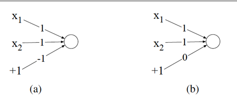
> the most simple NN is also called perceptron.

Let’s suppose we have a neuron with the following weight vector and bias:
w = [0.2, 0.3, 0.9]
b = 0.5
What would this neuron do with the following input vector:
x = [0.5, 0.6, 0.1]
The resulting output y would be:

y=sigmoid(wx+b)=1/1+e-(wx+b)=1/1+e-(0.5 * 0.2+ 0.6 * 0.3+ 0.1 * 0.9+0.5)=e-0.87=0.7

In practice, the sigmoid is not commonly used as an activation function.
A tanh function is very similar but almost always better; tanh is a variant of the sigmoid that ranges from -1 to +1
The simplest activation function, and perhaps the most commonly used, is the rectified linear unit (ReLU) [線性整流函數].

# The XOR Problem

AND and OR can be solve by the perceptron.
It turns out, however, that it’s not possible to build a perceptron to compute logical XOR!

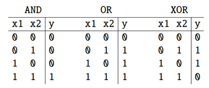
The reason why a multilayer neural network (MLNN) with nonlinear activation functions can solve the XOR problem is that it introduces nonlinear transformations, which can project data that cannot be separated linearly into a new space where it becomes linearly separable.

# Back-propagation

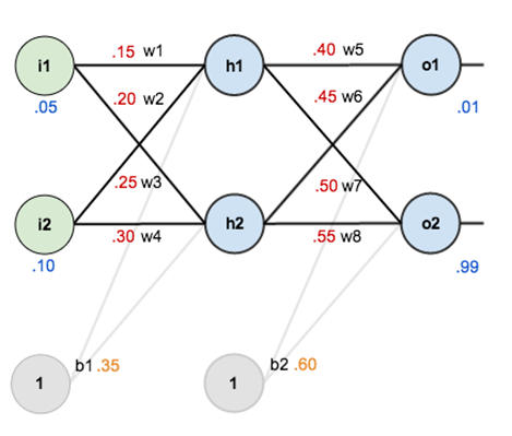
The net input of h1 : **net(h1)** = w1 * i1 + w2 * i2 + b1 * 1 = 0.15 * 0.05 + 0.2 * 0.1 + 0.35 * 1 = 0.3775
The output of h1 : **outh1** = sigmoid(h1) = 1/(1+ⅇ^(−0.3775) )=0.593269992
同理可得**outh2** = sigmoid(h2)>> 0.05 * 0.25 + 0.1 * 0.3 + 0.35 = 0.3925, sigmoid(0.3925) = 0.59684378
往下一層，我們也可以得到 neto1, neto2, **outo1** = 0.75136507, and **outo2** = 0.772928465

Calculate total error:
For simplicity, mean square error is used. That is, Etotal = ∑1/2 (𝑦−𝑦 ̂)^2 = Eo1 + Eo2
Because y01 = 0.01 and ŷo1 = outo1 = 0.75136507, Eo1 = 1/2 (0.01 – 0.75136507)^2 = 0.274811083
同理可得 Eo2 = 0.023560026
Thus, Etotal = Eo1 + Eo2 = 0.298371109

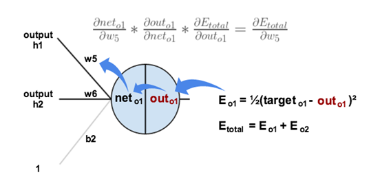
(𝜕𝐸_𝑡𝑜𝑡𝑎𝑙)/(𝜕𝑤_5 ) = **(𝜕𝐸_𝑡𝑜𝑡𝑎𝑙)/(𝜕𝑜𝑢𝑡_𝑜1 )** * (𝜕𝑜𝑢𝑡_𝑜1)/(𝜕𝑛𝑒𝑡_𝑜1 ) * (𝜕𝑛𝑒𝑡_𝑜1)/(𝜕𝑤_5 )
Etotal = Eo1 + Eo2 = 1/2 (y01 – outo1)^2 + 1/2 (y02 – outo2)^2
Thus, (𝜕𝐸_𝑡𝑜𝑡𝑎𝑙)/(𝜕𝑜𝑢𝑡_𝑜1 ) = 2 * 1/2 * (y01 – outo1) * -1 + 0 = - (y01 – outo1) = **0.74136507**

(𝜕𝐸_𝑡𝑜𝑡𝑎𝑙)/(𝜕𝑤_5 ) = (𝜕𝐸_𝑡𝑜𝑡𝑎𝑙)/(𝜕𝑜𝑢𝑡_𝑜1 ) * **(𝜕𝑜𝑢𝑡_𝑜1)/(𝜕𝑛𝑒𝑡_𝑜1 )** * (𝜕𝑛𝑒𝑡_𝑜1)/(𝜕𝑤_5 )
Since outo1 = 1/(1+ⅇ^(−𝑛𝑒𝑡_𝑜1 ) ), (𝜕𝑜𝑢𝑡_𝑜1)/(𝜕𝑛𝑒𝑡_𝑜1 ) = outo1 * (1 – outo1) = 0.75136507 * (1-0.75136507) = **0.186815602**

**Wiki: the partial derivative of the logistic function**

(𝜕𝐸_𝑡𝑜𝑡𝑎𝑙)/(𝜕𝑤_5 ) = (𝜕𝐸_𝑡𝑜𝑡𝑎𝑙)/(𝜕𝑜𝑢𝑡_𝑜1 ) * (𝜕𝑜𝑢𝑡_𝑜1)/(𝜕𝑛𝑒𝑡_𝑜1 ) * **(𝜕𝑛𝑒𝑡_𝑜1)/(𝜕𝑤_5 )**
Since neto1 = w5*outh1+w6*outh2+b2*1, (𝜕𝑛𝑒𝑡_𝑜1)/(𝜕𝑤_5 ) = outh1 = **0.593269992**

> (𝜕𝐸_𝑡𝑜𝑡𝑎𝑙)/(𝜕𝑤_5 ) = (𝜕𝐸_𝑡𝑜𝑡𝑎𝑙)/(𝜕〖𝑜𝑢𝑡_𝑜1 ) * (𝜕𝑜𝑢𝑡_𝑜1)/(𝜕𝑛𝑒𝑡_𝑜1 ) * (𝜕𝑛𝑒𝑡_𝑜1)/(𝜕𝑤_5 ) = 0.74136507 * 0.186815602 * 0.593269992 = 0.082167041

Update w5:
W(t+1)5 = w(t)5 - η * (𝜕𝐸_𝑡𝑜𝑡𝑎𝑙)/(𝜕𝑤_5 ) = 0.4 – 0.5 * 0.082167041 = 0.35891648
Similarly, we have
* W(t+1)6 =0.408666186,
* W(t+1)7 =0.511301270, and
* W(t+1)8 =0.561370121.

# Deep learning architectures

Deep learning architectures are based on a sequence of heterogeneous layers which perform different operations organized in a computational graph.
The most interesting applications have been possible thanks to this stacking strategy, where the number of variable elements (weights and biases) can easily reach over 10 million; therefore, the ability to capture small details and generalize them exceeds any expectations.

The most important layer types
**Fully connected layers**
A fully connected (sometimes called dense) layer is made up of n neurons and each of them receives all the output values coming from the previous layer
The softmax activation function allows having an output vector where each element is the probability of a class (and the sum of all outputs is always normalized to 1.0)
This type of output can easily be trained using a cross-entropy loss function.

**Convolutional layers（CNN; 卷積神經網路）**
2012 年之後最夯的影像辨識模型
it will output numbers that describe the probability of the image being a certain class (.80 for cat, .15 for dog, .05 for bird, etc).
is able perform image classification by looking for low level features such as edges and curves, and then building up to more abstract concepts through a series of convolutional layers.
Thus, various types of detectors (or filters) are required.

**Dropout layers**
A dropout layer is used to prevent overfitting of the network by randomly setting a fixed number of input elements to 0.
This layer is adopted during the training phase, but it’s normally deactivated during test, validation, and production phases.
Dropout is very useful in very big models, where it increases the overall performance and reduces the risk of freezing some weights and overfitting the model

**Recurrent neural networks**
A recurrent layer is made up of particular neurons that present recurrent connections so as to bind the state at time t to its previous values (in general, only one).
This category of computational cells is particularly useful when it's necessary to capture the temporal dynamics of an input sequence.

In Tensorflow, building the neural network requires configuring the layers of the model, then compiling the model.
To configure the model, Tensorflow 支援至少兩種建立方式:
* **Sequential APIs**: Easy, but limited, cannot handle multiple inputs/outputs, cannot share layers
> A Sequential model is appropriate for a plain stack of layers where each layer has exactly one input tensor and one output tensor.
* **Functional APIs**: Powerful, but complex
> Any of your layers has multiple inputs or multiple outputs

import tensorflow as tf
from tensorflow.keras.models import Sequential
from tensorflow.keras.layers import Dense

# 建立 Sequential 模型
model = Sequential([
    Dense(64, activation='relu', input_shape=(10,)),  # 第一層，輸入特徵為 10
    Dense(32, activation='relu'),                     # 第二層
    Dense(1, activation='sigmoid')                    # 輸出層，用於二分類問題
])

# 編譯模型
model.compile(optimizer='adam', loss='binary_crossentropy', metrics=['accuracy'])

# 概述模型
model.summary()

┏━━━━━━━━━━━━━━━━━━━━━━━━━━━━━━━━━┳━━━━━━━━━━━━━━━━━━━━━━━━┳━━━━━━━━━━━━━━━┓
┃ Layer (type)                    ┃ Output Shape           ┃       Param # ┃
┡━━━━━━━━━━━━━━━━━━━━━━━━━━━━━━━━━╇━━━━━━━━━━━━━━━━━━━━━━━━╇━━━━━━━━━━━━━━━┩
│ dense_13 (Dense)                │ (None, 64)             │           704 │
├─────────────────────────────────┼────────────────────────┼───────────────┤
│ dense_14 (Dense)                │ (None, 32)             │         2,080 │
├─────────────────────────────────┼────────────────────────┼───────────────┤
│ dense_15 (Dense)                │ (None, 1)              │            33 │
└─────────────────────────────────┴────────────────────────┴───────────────┘

import tensorflow as tf
from tensorflow.keras.layers import Input, Dense, concatenate
from tensorflow.keras.models import Model

# 定義輸入
input1 = Input(shape=(10,))
input2 = Input(shape=(20,))

# 定義層
x1 = Dense(64, activation='relu')(input1)
x2 = Dense(64, activation='relu')(input2)

# 合併層
merged = concatenate([x1, x2])

# 添加後續層
x = Dense(32, activation='relu')(merged)
output = Dense(1, activation='sigmoid')(x)

# 建立模型
model = Model(inputs=[input1, input2], outputs=output)

# 編譯模型
model.compile(optimizer='adam', loss='binary_crossentropy', metrics=['accuracy'])

# 概述模型
model.summary()

┏━━━━━━━━━━━━━━━━━━━━━┳━━━━━━━━━━━━━━━━━━━┳━━━━━━━━━━━━┳━━━━━━━━━━━━━━━━━━━┓
┃ Layer (type)        ┃ Output Shape      ┃    Param # ┃ Connected to      ┃
┡━━━━━━━━━━━━━━━━━━━━━╇━━━━━━━━━━━━━━━━━━━╇━━━━━━━━━━━━╇━━━━━━━━━━━━━━━━━━━┩
│ input_layer_6       │ (None, 10)        │          0 │ -                 │
│ (InputLayer)        │                   │            │                   │
├─────────────────────┼───────────────────┼────────────┼───────────────────┤
│ input_layer_7       │ (None, 20)        │          0 │ -                 │
│ (InputLayer)        │                   │            │                   │
├─────────────────────┼───────────────────┼────────────┼───────────────────┤
│ dense_16 (Dense)    │ (None, 64)        │        704 │ input_layer_6[0]… │
├─────────────────────┼───────────────────┼────────────┼───────────────────┤
│ dense_17 (Dense)    │ (None, 64)        │      1,344 │ input_layer_7[0]… │
├─────────────────────┼───────────────────┼────────────┼───────────────────┤
│ concatenate         │ (None, 128)       │          0 │ dense_16[0][0],   │
│ (Concatenate)       │                   │            │ dense_17[0][0]    │
├─────────────────────┼───────────────────┼────────────┼───────────────────┤
│ dense_18 (Dense)    │ (None, 32)        │      4,128 │ concatenate[0][0] │
├─────────────────────┼───────────────────┼────────────┼───────────────────┤
│ dense_19 (Dense)    │ (None, 1)         │         33 │ dense_18[0][0]    │
└─────────────────────┴───────────────────┴────────────┴───────────────────┘

iris資料集實作

import numpy as np
import tensorflow as tf
from tensorflow.keras import Sequential
from tensorflow.keras.layers import Dense
from sklearn.datasets import load_iris
from sklearn.model_selection import train_test_split
from sklearn.preprocessing import OneHotEncoder

import matplotlib.pyplot as plt

from sklearn.datasets import load_iris
from sklearn.model_selection import train_test_split
from sklearn.preprocessing import OneHotEncoder

# 加載 iris 資料集
iris = load_iris()
X = iris.data
Y = iris.target.reshape(-1, 1)

# 使用 OneHotEncoder 進行標籤的 One-Hot 編碼
encoder = OneHotEncoder(sparse_output=False)
Y = encoder.fit_transform(Y)

# 分割資料集為訓練集和測試集
X_train, X_test, Y_train, Y_test = train_test_split(X, Y, test_size=0.2, random_state=42)

model = Sequential()
model.add(Dense(10, activation='relu', input_shape=(4,)))  # 第一層有 10 個神經元，輸入特徵為 4
model.add(Dense(10, activation='relu'))  # 第二層有 10 個神經元
model.add(Dense(3, activation='softmax'))  # 輸出層有 3 個神經元，對應 3 個類別，使用 softmax 激活函數

model.compile(optimizer='adam', loss='categorical_crossentropy', metrics=['accuracy'])

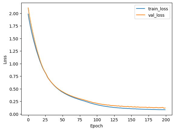
history = model.fit(X_train, Y_train, epochs=200, validation_data=(X_test, Y_test))

# 可視化訓練過程
plt.plot(history.history['loss'], label='train_loss')
plt.plot(history.history['val_loss'], label='val_loss')
plt.ylabel('Loss')
plt.xlabel('Epoch')
plt.legend()
plt.show()

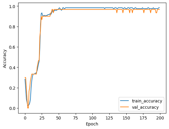
plt.plot(history.history['accuracy'], label='train_accuracy')
plt.plot(history.history['val_accuracy'], label='val_accuracy')
plt.ylabel('Accuracy')
plt.xlabel('Epoch')
plt.legend()
plt.show()

Epoch 190/200
4/4 ━━━━━━━━━━━━━━━━━━━━ 0s 13ms/step - accuracy: 0.9827 - loss: 0.0626 - val_accuracy: 0.9667 - val_loss: 0.1209
Epoch 191/200
4/4 ━━━━━━━━━━━━━━━━━━━━ 0s 12ms/step - accuracy: 0.9881 - loss: 0.0810 - val_accuracy: 0.9667 - val_loss: 0.1210
Epoch 192/200
4/4 ━━━━━━━━━━━━━━━━━━━━ 0s 15ms/step - accuracy: 0.9712 - loss: 0.0784 - val_accuracy: 0.9667 - val_loss: 0.1234
Epoch 193/200
4/4 ━━━━━━━━━━━━━━━━━━━━ 0s 12ms/step - accuracy: 0.9712 - loss: 0.0835 - val_accuracy: 0.9667 - val_loss: 0.1235
Epoch 194/200
4/4 ━━━━━━━━━━━━━━━━━━━━ 0s 11ms/step - accuracy: 0.9848 - loss: 0.0627 - val_accuracy: 0.9667 - val_loss: 0.1218
Epoch 195/200
4/4 ━━━━━━━━━━━━━━━━━━━━ 0s 16ms/step - accuracy: 0.9671 - loss: 0.0970 - val_accuracy: 0.9333 - val_loss: 0.1268
Epoch 196/200
4/4 ━━━━━━━━━━━━━━━━━━━━ 0s 14ms/step - accuracy: 0.9733 - loss: 0.0979 - val_accuracy: 0.9333 - val_loss: 0.1292
Epoch 197/200
4/4 ━━━━━━━━━━━━━━━━━━━━ 0s 14ms/step - accuracy: 0.9733 - loss: 0.0914 - val_accuracy: 0.9667 - val_loss: 0.1245
Epoch 198/200
4/4 ━━━━━━━━━━━━━━━━━━━━ 0s 17ms/step - accuracy: 0.9765 - loss: 0.0706 - val_accuracy: 0.9667 - val_loss: 0.1140
Epoch 199/200
4/4 ━━━━━━━━━━━━━━━━━━━━ 0s 15ms/step - accuracy: 0.9767 - loss: 0.1017 - val_accuracy: 0.9667 - val_loss: 0.1138
Epoch 200/200
4/4 ━━━━━━━━━━━━━━━━━━━━ 0s 21ms/step - accuracy: 0.9767 - loss: 0.0986 - val_accuracy: 0.9667 - val_loss: 0.1167


test_loss, test_acc = model.evaluate(X_test, Y_test)
print(f"Test accuracy: {test_acc:.4f}")

1/1 ━━━━━━━━━━━━━━━━━━━━ 0s 32ms/step - accuracy: 0.9667 - loss: 0.1167
Test accuracy: 0.9667

import numpy as np

# 假設 predictions 和 true_classes 已經定義
predictions = model.predict(X_test)
predicted_classes = np.argmax(predictions, axis=1)
true_classes = np.argmax(Y_test, axis=1)

# 確保兩個列表的長度相同
assert len(predicted_classes) == len(true_classes)

# 打印對齊的結果
print("Predicted classes: ", end="")
for i in predicted_classes:
    print(f"{i:2d} ", end="")
print()

print("  True classes:   ", end="")
for i in true_classes:
    print(f"{i:2d} ", end="")
print()

> 1/1 ━━━━━━━━━━━━━━━━━━━━ 0s 51ms/step
> Predicted classes: 1 0 2 1 1 0 1 2 2 1 2 0 0 0 0 1 2 1 1 2 0 2 0 2 2 2 2 2 0 0
> True classes: 1 0 2 1 1 0 1 2 1 1 2 0 0 0 0 1 2 1 1 2 0 2 0 2 2 2 2 2 0 0