# Linear SVM

"Find the line that best separates the training data."(SVM 的目標是找到一條能夠正確分類訓練的分類線)

"Among all such lines, pick the one that maximizes the margin, which is the distance to the points closest to it."(選擇與分類線距離最遠的點作為support vectors)

"The closest points that determine this line are known as support vectors, and the distance between these points and the line is known as the margin."(2倍support vectors與hyperline之間的距離稱為Margin).


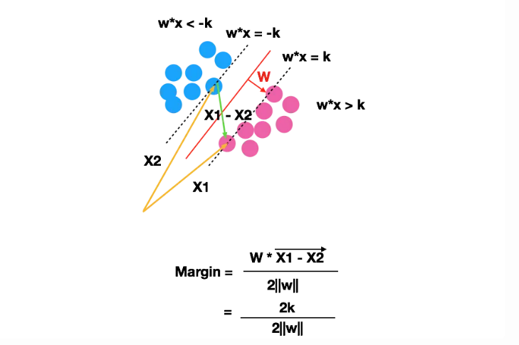
假設𝑤=[2,3],𝑥1=[1,5],𝑥2=[4,1]，並且𝑘=1：

計算範數∥𝑤∥：∥𝑤∥=開根號(2^2 + 3^2)=根號(4+9)=根號(13)

計算𝑥1−𝑥2：
𝑥1−𝑥2=[1−4,5−1]=[−3,4]

計算內積𝑤⋅(𝑥1−𝑥2)=[2,3]⋅[−3,4]=2×(−3)+3×4=−6+12=6

計算 Margin：= 6/2根號(13) = 3/根號(13)

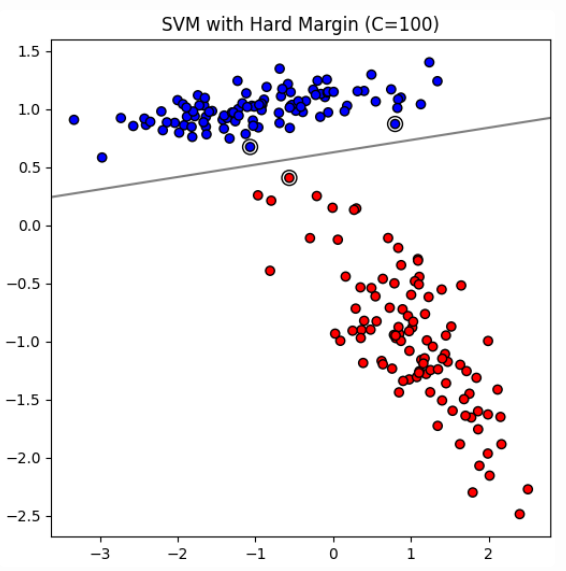
# Hard Margin
In ideal scenarios where data is perfectly linearly separable, SVM can employ a hard margin approach. This means that the algorithm seeks to find a hyperplane that separates the data without any misclassification. The hard margin SVM does not tolerate any errors, and every data point must be correctly classified with the widest possible margin.

* In hard margin SVM, the C value is theoretically infinite. This means that the model imposes an infinite penalty on misclassification, ensuring that no points are misclassified.
* Limitations: Highly sensitive to noise and outliers, making it less practical for real-world data that often contains imperfections.


# Soft Margin
In real-world scenarios, data often contains noise or overlap between classes, making perfect linear separability impossible. To address this, SVMs introduce a soft margin, which allows some points to be on the wrong side of the margin or even misclassified. The idea is to find a balance between maximizing the margin and minimizing classification errors.

High 𝐶 Value:

* When 𝐶 is large, the SVM prioritizes minimizing classification errors over having a wide margin.
* The decision boundary will fit the training data more closely, potentially leading to a smaller margin.
* This can result in better classification performance on the training data but might cause overfitting, reducing generalization to new data.

Low 𝐶 Value:
* When 𝐶 is small, the SVM allows more classification errors in the training data to achieve a wider margin.
* The decision boundary will be smoother and less sensitive to individual data points.
* This can improve generalization to new data but might result in a higher error rate on the training data.


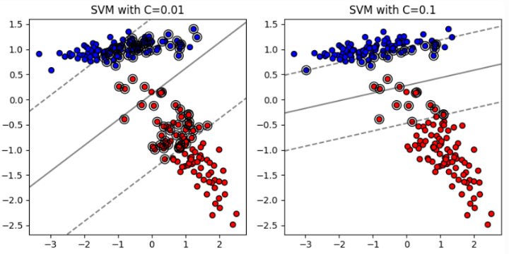
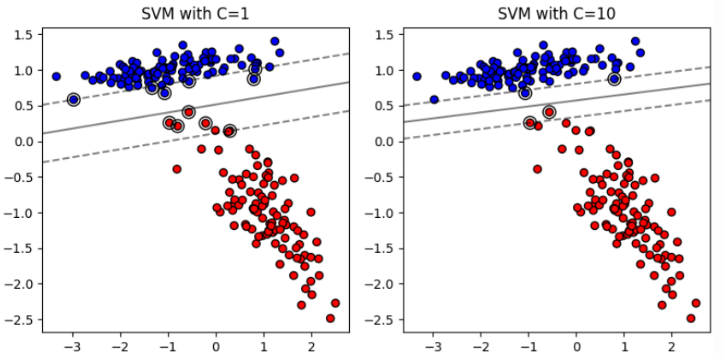
By adjusting the parameter C, you can control the **tradeoff** between having a wide margin and correctly classifying the training data, thereby influencing the model's complexity and generalization ability.(Trade-off problem,C越大,margin越小，反之)

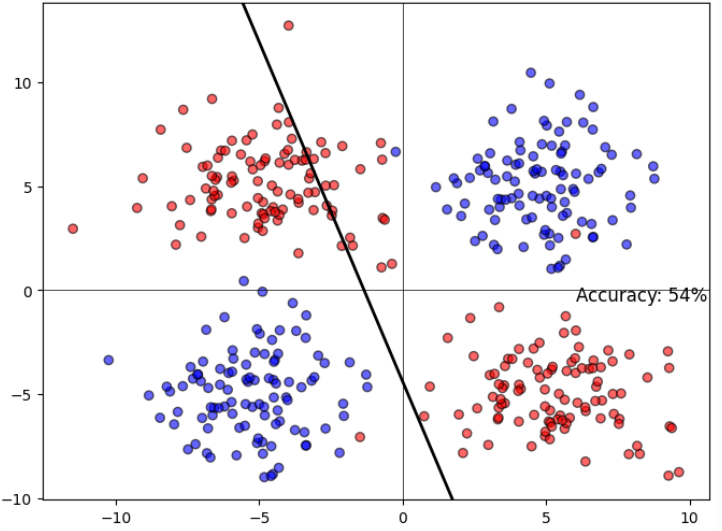
# Non-linear SVM

Non-linearly Separable Data
當我們一樣使用linear的方式來解決Non-linearly Separable Data，就會發現效果很差

SVM can solve non-linearity by projecting the data into a space where it is linearly separable and find a hyperplane in this space!
Let's project the original two-dimensional space to three-dimensional space and see what the data looks like:

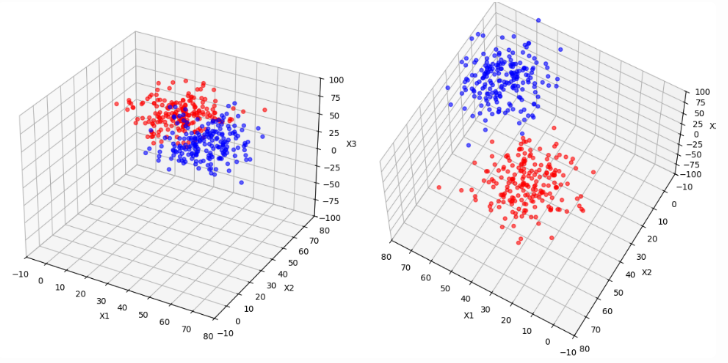
可以發現，只要將data投影到更高維的空間就可以變得更linearly separable

"How did I know what space to project the data onto (or which 𝜙(𝑥𝑖)is better)?"

* In General, Hard to Know: Determining the exact transformation (or mapping function 𝜙) that will make the data linearly separable can be difficult without prior knowledge of the data structure.
* Cover’s Theorem Insight: However, according to Cover's theorem, data is more likely to be linearly separable when projected onto higher dimensions.

So project the data first and then run the SVM?
* The fact is you ask the SVM to do the projection for you.
* SVM use something called kernels to do these projections, and these are pretty fast

**只需要選擇一個合適的核函數（kernel function），SVM會自動利用該核函數在訓練過程中進行投影和計算**

## Dot Product

假設我們有兩個點 𝑥 和 𝑧 ，它們在原始空間中的坐標分別是 𝑥 = [ 𝑥 1 , 𝑥 2 ] 和 𝑧 = [ 𝑧 1 , 𝑧 2 ]。如果我們想將這兩個點投影到三維空間，投影函數為：
ϕ(x)=[x1​,x2​,x^2​+ x^2​]
ϕ(z)=[z1​,z2​,z^2​+ z^2​]

我們需要計算這兩個投影後向量的內積：𝜙(𝑥)⋅𝜙(𝑧)=(𝑥1⋅𝑧1)+(𝑥2⋅𝑧2)+((𝑥^2 + 𝑥^2) ⋅ (𝑧^2 + 𝑧^2))

這裡涉及到的計算步驟包括：
1. 𝑥1⋅𝑧1
1. 𝑥2⋅𝑧2
1. 𝑥^2 ⋅ 𝑧^2
1. 𝑥^2 ⋅ 𝑧^2
1. 𝑥^2 ⋅ 𝑧^2
1. 𝑥^2 ⋅ 𝑧^2
1. 將以上結果相加

這樣的計算隨著維度增加，計算量會迅速增大。

## Kernel Function

K(x,z)=exp(−γ∥x−z∥^2)

其中∥𝑥−𝑧∥^2是歐幾里得距離的平方。我們只需要計算兩個點之間的歐幾里得距離平方，再做一次指數運算即可。具體步驟為：

1. 計算歐幾里得距離平方：∥𝑥−𝑧∥^2 = (𝑥1−𝑧1)^2 + (𝑥2−𝑧2)^2
1. 做指數運算：exp⁡(−𝛾∥𝑥−𝑧∥^2)

這裡的計算步驟包括：
1. (𝑥1−𝑧1)^2
1. (𝑥2−𝑧2)^2
1. 將以上結果相加
1. 對結果進行指數運算

可以看到，這裡的計算量明顯比Dot Product投影內積要少得多。

# Summary

### Linear SVM

Linear kernal
* 文本分類：在文本分類中，使用 TF-IDF 或詞袋模型表示的文本數據通常是高維的。例如，對新聞文章進行分類（例如，體育、科技、政治），這類數據通常是線性可分的，因此使用線性核效果較好。
* 垃圾郵件分類：使用電子郵件的特徵（例如詞頻、關鍵詞出現等）來區分垃圾郵件和正常郵件，這類特徵數量通常非常多，適合使用線性核。

### Non-linear SVM

Polynomial Kernel
* 影像處理：在影像識別中，像素之間的關係可能是非線性的。例如，識別手寫字母時，不同筆劃之間的關係可能不是線性的，多項式核可以捕捉到這些複雜的關係。
* 股票價格預測：使用歷史價格和其他市場指標來預測股票價格，這些特徵之間的關係通常是非線性的。

Radial Basis Function Kernel (RBF)
* 手寫數字識別：MNIST 手寫數字數據集，數字的形狀和結構高度多樣且具有非線性關係，RBF 核在這種情況下表現優異。
* 醫學數據分類：如癌症診斷數據，特徵之間的關係複雜且非線性，使用 RBF 核可以有效地捕捉這些關係。

Sigmoid Kernel
* 生物資料處理：在某些基因表達數據中，特徵之間的關係可能類似於神經網絡中的激活函數，使用 Sigmoid 核可以有效地捕捉這些關係。
* 社交網絡資料分析：在分析社交網絡數據（例如，朋友關係、互動次數等）時，這些數據的分佈可能呈現非線性，Sigmoid 核可以用來模擬這種非線性。

RBF是最常用的核函數，因為它在大多數情況下都能表現不錯。

程式碼:

import pandas as pd
import numpy as np
import matplotlib.pyplot as plt
from sklearn import datasets
from sklearn.model_selection import train_test_split
from sklearn.preprocessing import StandardScaler
from sklearn.decomposition import PCA
from sklearn.svm import SVC
from sklearn.metrics import accuracy_score

# 載入 Iris 資料集
iris = datasets.load_iris()

# 將資料轉換成 DataFrame
df = pd.DataFrame(data=iris.data, columns=iris.feature_names)
df['target'] = iris.target

# # 顯示前三筆完整數據
# print(df.head(3))
feature_names = iris.feature_names
# 類別名稱
target_names = iris.target_names

print("特徵名稱：", feature_names)
print("類別名稱：", target_names)

# 劃分特徵變數和目標變數
X = df.drop(columns=['target'])
y = df['target']

# 劃分訓練集和測試集
X_train, X_test, y_train, y_test = train_test_split(X, y, test_size=0.2, random_state=42)

# 標準化特徵
scaler = StandardScaler()
X_train = scaler.fit_transform(X_train)
X_test = scaler.transform(X_test)

# 使用 PCA 將數據降維到二維
pca = PCA(n_components=2)
X_train_pca = pca.fit_transform(X_train)
X_test_pca = pca.transform(X_test)

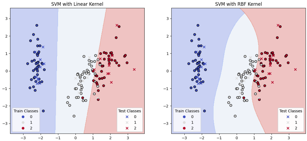
# 訓練 SVM 模型（線性核）
linear_svc = SVC(kernel='linear', probability=True, random_state=42)
linear_svc.fit(X_train_pca, y_train)

# 使用線性核模型進行預測
y_pred_linear = linear_svc.predict(X_test_pca)
y_prob_linear = linear_svc.predict_proba(X_test_pca)

# 輸出線性核模型的預測結果及其概率

print("線性核模型的準確率：", accuracy_score(y_test, y_pred_linear))

# 訓練 SVM 模型（非線性核，例如 RBF）
rbf_svc = SVC(kernel='rbf', probability=True, random_state=42)
rbf_svc.fit(X_train_pca, y_train)

# 使用非線性核模型進行預測
y_pred_rbf = rbf_svc.predict(X_test_pca)
y_prob_rbf = rbf_svc.predict_proba(X_test_pca)

# 輸出非線性核模型的預測結果及其概率

print("非線性核模型的準確率：", accuracy_score(y_test, y_pred_rbf))

特徵名稱： ['sepal length (cm)', 'sepal width (cm)', 'petal length (cm)', 'petal width (cm)']
類別名稱： ['setosa' 'versicolor' 'virginica']
線性核模型的準確率： 0.9
非線性核模型的準確率： 0.9

# 創建網格來評估模型
h = .02  # 步長
x_min, x_max = X_train_pca[:, 0].min() - 1, X_train_pca[:, 0].max() + 1
y_min, y_max = X_train_pca[:, 1].min() - 1, X_train_pca[:, 1].max() + 1
xx, yy = np.meshgrid(np.arange(x_min, x_max, h),
                     np.arange(y_min, y_max, h))

# 繪製決策邊界和數據點
def plot_decision_boundary(model, ax, title, X_train_pca, y_train, X_test_pca, y_test):
    # 預測網格中的每一點
    Z = model.predict(np.c_[xx.ravel(), yy.ravel()])
    Z = Z.reshape(xx.shape)

    # 繪製決策邊界
    ax.contourf(xx, yy, Z, alpha=0.3, cmap=plt.cm.coolwarm)

    # 繪製訓練數據點
    scatter_train = ax.scatter(X_train_pca[:, 0], X_train_pca[:, 1], c=y_train, cmap=plt.cm.coolwarm, edgecolor='k', marker='o', label='Train')

    # 繪製測試數據點
    scatter_test = ax.scatter(X_test_pca[:, 0], X_test_pca[:, 1], c=y_test, cmap=plt.cm.coolwarm, edgecolor='k', marker='x', label='Test')

    # 添加圖例
    legend1 = ax.legend(*scatter_train.legend_elements(), title="Train Classes", loc='lower left')
    legend2 = ax.legend(*scatter_test.legend_elements(), title="Test Classes", loc='lower right')
    ax.add_artist(legend1)
    ax.add_artist(legend2)

    # 設置圖形範圍和標題
    ax.set_xlim(xx.min(), xx.max())
    ax.set_ylim(yy.min(), yy.max())
    ax.set_title(title)

# 繪製圖形
fig, (ax1, ax2) = plt.subplots(1, 2, figsize=(14, 6))

plot_decision_boundary(linear_svc, ax1, 'SVM with Linear Kernel', X_train_pca, y_train, X_test_pca, y_test)
plot_decision_boundary(rbf_svc, ax2, 'SVM with RBF Kernel', X_train_pca, y_train, X_test_pca, y_test)

plt.show()